MTF EMA Traffic Light System Trend Alignment for ScalpersMTF EMA Traffic Light – Trend Bias System
This indicator is designed to help traders quickly identify high-probability trend alignment using multiple timeframes and EMAs.
It analyzes price relative to the 13 EMA and 55 EMA on:
1 Minute
5 Minute
15 Minute
1 Hour
4 Hour
Then it converts that data into a simple Traffic Light system to guide trade decisions.
🚦 How It Works
Each timeframe is classified as:
🟢 BULL – Price above both EMAs
🔴 BEAR – Price below both EMAs
🟡 MIXED – No clear direction
The system focuses on lower-timeframe alignment:
When 1m + 5m + 15m are aligned → Strong setup
When mixed → Caution
When misaligned → Stand aside
🟢 GREEN State (Full Trade Mode)
Triggered when:
✔ 1m, 5m, and 15m are all BULL → Long Bias
✔ 1m, 5m, and 15m are all BEAR → Short Bias
Rules:
Full position size
Trade with trend
Look for EMA pullbacks
Let winners run
🟡 YELLOW State (Caution Mode)
Triggered when:
✔ Lower timeframes are mixed
Rules:
Reduce size
Take quick profits
No holding
Defensive trading
🔴 RED State (No Trade)
Triggered when:
✔ No clear alignment
Rules:
Stay out
Mark key levels
Protect capital
📋 Dashboard Panel
The indicator displays a real-time table showing:
Each timeframe’s bias
Overall market state
Trade rules
This allows you to read market structure in seconds without switching charts.
🎯 Best Use
This tool works best for:
✔ Scalping
✔ Intraday trading
✔ Trend continuation setups
✔ EMA pullback strategies
Recommended for:
Forex
Indices
Gold
Crypto
⚠️ Risk Disclaimer
This indicator is a decision-support tool, not a guarantee of profits.
Always use:
Proper risk management
Stop losses
Personal trade rules
Never risk more than you can afford to lose.
Cerca negli script per "stop loss"

Bubble Risk ModelThe question of whether markets can be objectively assessed for overextension has occupied financial researchers for decades. Charles Kindleberger, in his seminal work "Manias, Panics, and Crashes" (1978), documented that speculative bubbles follow remarkably consistent patterns across centuries and asset classes. Yet identifying these patterns in real time remains notoriously difficult. The Bubble Risk Model attempts to address this challenge not by predicting crashes, but by systematically measuring the statistical characteristics that historically precede fragile market conditions.
The theoretical foundation draws from two distinct research traditions. The first is the work on regime-switching models pioneered by James Hamilton (1989), who demonstrated that economic time series often exhibit discrete shifts between different behavioral states. The second is the literature on tail risk and market fragility, most notably articulated by Nassim Taleb in "The Black Swan" (2007), which emphasizes that extreme events carry disproportionate importance and that traditional risk measures systematically underestimate their probability.
Rather than attempting to build a probabilistic model requiring assumptions about underlying distributions, the Bubble Risk Model operates as a deterministic state-inference system. This distinction matters. Lawrence Rabiner's foundational tutorial on Hidden Markov Models (1989) established the mathematical framework for inferring hidden states from observable data through Bayesian updating. The present model borrows the conceptual architecture of states and transitions but replaces probabilistic inference with rule-based logic. States are not computed through forward-backward algorithms but inferred through deterministic thresholds. This trade-off sacrifices theoretical elegance for practical robustness and interpretability.
The measurement framework rests on four empirically grounded components. The first captures trailing twelve-month returns, reflecting the well-documented momentum effect identified by Jegadeesh and Titman (1993), who found that securities with strong past performance tend to continue outperforming over intermediate horizons. The second component measures trend persistence as the proportion of positive daily returns over a quarterly window, drawing on the research by Campbell and Shiller (1988) showing that price trends exhibit serial correlation that deviates from random walk assumptions. The third normalizes the distance between current prices and their long-term moving average by volatility, addressing the cross-sectional comparability problem noted by Fama and French (1992) when analyzing assets with different variance characteristics. The fourth component calculates return efficiency as the ratio of returns to realized volatility, a concept related to the Sharpe ratio but stripped of distributional assumptions that often fail in practice.
The aggregation methodology deliberately prioritizes worst-case scenarios. Rather than averaging component scores, the model uses quantile-based aggregation with an explicit tail penalty. This design choice reflects the asymmetric error costs in bubble detection: failing to identify fragility carries greater consequences than occasional false positives. The approach aligns with the precautionary principle advocated by Taleb and colleagues in their work on fragility and antifragility (2012), which argues that systems exposed to tail risks require conservative assessment frameworks.
Normalization presents a particular challenge. Raw metrics like year-over-year returns are not directly comparable across asset classes with different volatility profiles. The model addresses this through percentile ranking over multiple historical windows, typically two and five years. This dual-window approach provides regime stability, preventing the normalization from adapting too quickly during extended bull markets where elevated readings become statistically normal. The methodology draws on the concept of lookback bias documented by Lo and MacKinlay (1990), who demonstrated that single-window statistical measures can produce misleading results when market regimes shift.
The state machine introduces controlled inertia into the system. Once the model enters a particular state, transitions become progressively more difficult as the state matures. This transition resistance mechanism prevents rapid oscillation near threshold boundaries, a problem that plagues many indicator-based systems. The concept parallels the hysteresis effects described in economic literature by Dixit (1989), where systems exhibit path dependence and resist returning to previous states even when underlying conditions change.
Volatility regime detection adds contextual interpretation. Research by Engle (1982) on autoregressive conditional heteroskedasticity established that volatility clusters, with periods of high volatility tending to follow other high-volatility periods. The model scales its maturity thresholds inversely with volatility: in calm markets, states mature slowly and persist longer; in turbulent markets, information decays faster and states become more transient. This adaptive behavior reflects the empirical observation that low-volatility environments often precede significant market dislocations, as documented by Brunnermeier and Pedersen (2009) in their work on liquidity spirals.
The confidence metric addresses internal model consistency. When individual components diverge substantially, the overall score becomes less reliable regardless of its absolute level. This approach draws on ensemble methods in machine learning, where disagreement among predictors signals increased uncertainty. Dietterich (2000) provides theoretical justification for this principle, demonstrating that ensemble disagreement correlates with prediction error.
Distribution drift detection monitors whether the model's calibration remains valid. By comparing recent score distributions to longer historical baselines, the model can identify when market structure has shifted sufficiently to potentially invalidate its historical percentile rankings. This self-diagnostic capability reflects the concern raised by Andrews (1993) about parameter instability in time series models, where structural breaks can render previously estimated relationships unreliable.
The cross-asset analysis extends the framework beyond individual securities. By calculating scores for multiple asset classes simultaneously and measuring their correlation, the model distinguishes between idiosyncratic overextension affecting a single asset and systemic conditions affecting markets broadly. This differentiation matters for portfolio construction, as documented by Longin and Solnik (2001), who found that correlations between international equity markets increase significantly during periods of market stress.
Several limitations deserve explicit acknowledgment. The model cannot identify timing. Overextended conditions can persist far longer than rational analysis might suggest, a phenomenon documented by Shiller (2000) in his analysis of speculative episodes. The model provides no mechanism for determining when fragile conditions will resolve. Additionally, the cross-asset analysis lacks lead-lag detection, meaning it cannot distinguish whether assets became overextended simultaneously or sequentially. Finally, the rule-based nature of state inference means the model cannot express graduated probability assessments; states are discrete rather than continuous.
The philosophical stance underlying the model is one of epistemic humility. It does not claim to identify bubbles definitively or predict their collapse. Instead, it provides a systematic framework for measuring characteristics that have historically been associated with fragile market conditions. The distinction between information and action remains the user's responsibility. States describe current conditions; how to respond to those conditions requires judgment that no quantitative model can provide.
Practical guide for traders
This section translates the model's outputs into actionable intelligence for both retail traders managing personal portfolios and professional traders operating within institutional frameworks. The interpretation differs not in kind but in scale and consequence.
Understanding the score
The primary output is a continuous score ranging from zero to one. Lower scores indicate elevated bubble risk; higher scores suggest more sustainable market conditions. This inverse relationship may seem counterintuitive but reflects the model's construction: it measures how extreme current conditions are relative to historical norms, with extremity mapping to fragility.
A score above 0.50 generally indicates normal market conditions where standard investment approaches remain appropriate. Scores between 0.30 and 0.50 represent an elevated zone where caution is warranted but not alarm. Scores below 0.30 enter the extreme territory where historical precedent suggests increased fragility. These thresholds are not magical boundaries but represent statistical rarity: a score below 0.30 indicates conditions that occur in roughly the bottom quintile of historical observations.
For retail traders, a score in the normal range means continuing with established strategies without modification. In the elevated range, this might mean pausing new position additions while maintaining existing holdings. In the extreme range, retail traders should consider whether their portfolio could withstand a significant drawdown and whether their time horizon permits waiting for recovery. For professional traders, the score integrates into broader risk frameworks: normal conditions permit full risk budgets, elevated conditions might trigger reduced position sizing or tighter stop losses, and extreme conditions could warrant defensive positioning or increased hedging activity.
Reading the states
The model classifies conditions into three discrete states: Normal, Elevated, and Extreme. These states differ from the continuous score by incorporating persistence and transition resistance. A market can have a score temporarily dipping below 0.30 without triggering an Extreme state if the condition proves transient.
The Normal state indicates business as usual. Market conditions fall within historical norms across all measured dimensions. For retail traders, this means standard portfolio management applies. For professional traders, full strategy deployment remains appropriate with normal risk parameters.
The Elevated state signals heightened attention. At least one dimension of market behavior has moved outside normal ranges, though not to extreme levels. Retail traders should review portfolio concentration and ensure diversification remains intact. Professional traders might reduce leverage slightly, tighten risk limits, or increase monitoring frequency.
The Extreme state represents statistically rare conditions. Multiple dimensions show readings that historically occur infrequently. Retail traders should seriously evaluate whether they can tolerate potential drawdowns and consider reducing exposure to volatile assets. Professional traders should implement defensive protocols, potentially reducing gross exposure, increasing cash allocations, or adding protective positions.
Interpreting transitions
State transitions carry more information than states themselves. The model tracks whether conditions are entering, persisting in, or exiting particular states.
An Entry into Extreme represents the most important signal. It indicates a regime shift from normal or elevated conditions into territory associated with historical fragility. For retail traders, this warrants immediate portfolio review. For professional traders, this typically triggers predefined defensive protocols.
Persistence in a state indicates stability. Whether Normal or Extreme, persistence suggests the current regime has become established. For retail traders, persistence in Extreme over extended periods actually reduces immediate concern; the dangerous moment was the entry, not the continuation. For professional traders, persistent Extreme states require maintained vigilance but do not necessarily demand additional action beyond what the initial entry triggered.
An Exit from Extreme suggests improving conditions. For retail traders, this might warrant cautious return to normal positioning over time. For professional traders, exits permit gradual normalization of risk budgets, though institutional memory typically counsels slower reentry than the mathematical signal might suggest.
Duration and its meaning
The model distinguishes between Tactical, Accelerating, and Structural durations in critical zones.
Tactical duration (10-39 bars in critical territory) represents short-term overextension. Many Tactical episodes resolve without significant market disruption. Retail traders should note the condition but need not take dramatic action. Professional traders might implement modest hedges or reduce marginal positions.
Accelerating indicates Tactical duration combined with actively deteriorating scores. This combination historically precedes more significant corrections. Retail traders should consider lightening positions in their most volatile holdings. Professional traders typically implement more substantial hedges.
Structural duration (40+ bars in critical territory) indicates persistent overextension that has become a market feature rather than a temporary condition. Paradoxically, Structural conditions are both more concerning and less immediately actionable than Accelerating conditions. The market has demonstrated ability to sustain extreme readings. Retail traders should maintain heightened awareness but recognize that timing remains impossible. Professional traders often find Structural conditions require strategy adaptation rather than simple defensive positioning.
Confidence and what it tells you
The Confidence reading indicates internal model consistency. High confidence means all four underlying components agree in their assessment. Low confidence means components diverge significantly.
High confidence combined with Extreme state represents the clearest signal. The model is both indicating fragility and agreeing with itself about that assessment. Retail and professional traders alike should treat this combination with maximum seriousness.
Low confidence in any state reduces signal reliability. For retail traders, low confidence suggests waiting for clearer conditions before making significant portfolio changes. For professional traders, low confidence warrants increased skepticism about the score and potentially reduced position sizing in either direction.
Alignment and model health
The Alignment indicator monitors whether the model's calibration remains valid relative to recent market behavior.
Good alignment means recent score distributions match longer-term historical patterns. The model's percentile rankings remain meaningful. Both retail and professional traders can interpret scores at face value.
Degraded alignment indicates that recent market behavior has shifted somewhat from historical norms. Scores remain interpretable but with reduced precision. Retail traders should apply wider uncertainty bands to their interpretation. Professional traders might reduce position sizing slightly or require additional confirmation before acting.
Poor alignment signals significant distribution shift. The model may be comparing current conditions to an increasingly irrelevant historical baseline. Retail traders should rely more heavily on other information sources during Poor alignment periods. Professional traders typically reduce model weight in their decision frameworks until alignment recovers.
Volatility regime context
The volatility regime provides essential context for score interpretation.
Low volatility combined with Extreme state creates maximum concern. Research consistently shows that low-volatility environments can precede significant market dislocations. The market's apparent calm masks underlying fragility. Retail traders should recognize that low volatility does not mean low risk; it often means compressed risk premiums that will eventually normalize, potentially violently. Professional traders typically maintain or increase defensive positioning despite the market's calm appearance.
High volatility combined with Extreme state is actually less immediately concerning than low volatility. The market has already acknowledged stress; risk premiums have expanded; potential sellers may have already sold. Retail traders should resist the urge to panic sell during high-volatility extremes, as much of the adjustment may have already occurred. Professional traders recognize that high-volatility extremes often represent better entry points than low-volatility extremes.
Normal volatility requires no regime adjustment to interpretation. Scores mean what they appear to mean.
Cross-asset analysis
When enabled, the model calculates scores for multiple asset classes simultaneously, enabling systemic versus idiosyncratic risk assessment.
Systemic risk (multiple assets in Extreme with high correlation) indicates market-wide fragility. Diversification benefits are reduced precisely when most needed. Retail traders should recognize that their portfolio's apparent diversification may not protect them during systemic events. Professional traders implement cross-asset hedges and consider tail-risk protection.
Broad risk (multiple assets in Extreme with low correlation) suggests widespread but potentially unrelated overextension. Diversification may still provide some protection. Retail traders can take modest comfort in genuine diversification. Professional traders analyze which assets might offer relative value.
Isolated risk (single asset in Extreme while others remain Normal) indicates asset-specific rather than market-wide conditions. Retail traders holding the affected asset should evaluate their position specifically. Professional traders may find relative value opportunities going long unaffected assets against the extended one.
Scattered risk represents a few assets showing elevation without clear pattern. This typically warrants monitoring rather than action for both retail and professional traders.
Parameter guidance
The Short Percentile parameter (default 504 bars, approximately two years) controls the shorter normalization window. Increasing this value makes the model more conservative, requiring more extreme readings to flag concern. Retail traders should generally leave this at default. Professional traders might increase it for assets with shorter reliable history.
The Long Percentile parameter (default 1260 bars, approximately five years) controls the longer normalization window. This provides regime stability. Again, default settings suit most applications.
The Critical Threshold (default 0.30) determines where the Extreme state boundary lies. Lowering this value makes the model less sensitive, flagging fewer Extreme conditions. Raising it increases sensitivity. Retail traders seeking fewer false alarms might lower this to 0.25. Professional traders seeking earlier warning might raise it to 0.35.
The Structural Duration parameter (default 40 bars) determines when Tactical conditions become Structural. Shorter values provide earlier Structural classification. Longer values require more persistence before reclassification.
The State Maturity and Transition Resistance parameters control how readily the model changes states. Higher values create more stable states with fewer transitions. Lower values create more responsive but potentially noisier state changes. Default settings balance responsiveness against stability.
The Adaptive Smoothing parameters control how the model filters noise. In extreme zones, longer smoothing periods reduce whipsaws but increase lag. In normal zones, shorter periods maintain responsiveness. Most traders should leave these at defaults.
What the model cannot do
The model cannot predict when overextended conditions will resolve. Markets can remain irrational longer than any trader can remain solvent, as the saying goes. Extended Extreme readings may persist for months or even years before any correction materializes.
The model cannot distinguish between healthy bull markets and dangerous bubbles in their early stages. Both initially appear as strong returns and positive momentum. The model begins flagging concern only when statistical extremity develops, which may occur well into an advance.
The model cannot account for fundamental changes in market structure. If a new paradigm genuinely justifies higher valuations (rare but not impossible), the model will continue flagging extremity against historical norms that may no longer apply. The Alignment indicator provides partial protection against this failure mode but cannot eliminate it.
The model cannot replace judgment. It provides systematic measurement of conditions that have historically preceded fragility. Whether and how to act on that measurement remains entirely the trader's responsibility. Retail traders must still evaluate their personal circumstances, time horizons, and risk tolerance. Professional traders must still integrate model output with fundamental analysis, portfolio constraints, and client mandates.
References
Andrews, D.W.K. (1993). Tests for Parameter Instability and Structural Change with Unknown Change Point. Econometrica, 61(4).
Brunnermeier, M.K., & Pedersen, L.H. (2009). Market Liquidity and Funding Liquidity. Review of Financial Studies, 22(6).
Campbell, J.Y., & Shiller, R.J. (1988). Stock Prices, Earnings, and Expected Dividends. Journal of Finance, 43(3).
Dietterich, T.G. (2000). Ensemble Methods in Machine Learning. Multiple Classifier Systems.
Dixit, A. (1989). Entry and Exit Decisions under Uncertainty. Journal of Political Economy, 97(3).
Engle, R.F. (1982). Autoregressive Conditional Heteroscedasticity with Estimates of the Variance of United Kingdom Inflation. Econometrica, 50(4).
Fama, E.F., & French, K.R. (1992). The Cross-Section of Expected Stock Returns. Journal of Finance, 47(2).
Hamilton, J.D. (1989). A New Approach to the Economic Analysis of Nonstationary Time Series and the Business Cycle. Econometrica, 57(2).
Jegadeesh, N., & Titman, S. (1993). Returns to Buying Winners and Selling Losers: Implications for Stock Market Efficiency. Journal of Finance, 48(1).
Kindleberger, C.P. (1978). Manias, Panics, and Crashes: A History of Financial Crises. Basic Books.
Lo, A.W., & MacKinlay, A.C. (1990). Data-Snooping Biases in Tests of Financial Asset Pricing Models. Review of Financial Studies, 3(3).
Longin, F., & Solnik, B. (2001). Extreme Correlation of International Equity Markets. Journal of Finance, 56(2).
Rabiner, L.R. (1989). A Tutorial on Hidden Markov Models and Selected Applications in Speech Recognition. Proceedings of the IEEE, 77(2).
Shiller, R.J. (2000). Irrational Exuberance. Princeton University Press.
Taleb, N.N. (2007). The Black Swan: The Impact of the Highly Improbable. Random House.
Taleb, N.N., & Douady, R. (2012). Mathematical Definition, Mapping, and Detection of (Anti)Fragility. Quantitative Finance, 13(11).

EvansThis is a simple math problem:
If your risk-reward ratio is 1:3.
Even if you lose 3 out of 4 trades (a win rate of only 25%), as long as you hit one big win, you'll still break even.
That extra bit of win rate is your pure profit.
📊 How to use it with LuxAlgo?
This script is your "skeleton," and LuxAlgo is your "muscle."
Hearing the green/red alarm: This means your system has detected a DEMA 9/20 crossover.
Confirm with the chart:
If LuxAlgo also shows a dark blue right-pointing arrow at this time, it represents a strong momentum 1:3 opportunity.
If the price is currently in the 0.618 Discount Zone, you must hold this trade.
Hearing the yellow alarm:
This is a reminder that the trend has changed. If you are already in profit but haven't reached a 1:3 ratio, you can consider manually reducing your position by half and then moving your stop loss to the entry point (Break Even), allowing the remaining profits to run without risk.

TradingView.To Strategy Template (with Dyanmic Alerts)Hello traders,
If you're tired of manual trading and looking for a solid strategy template to pair with your indicators, look no further.
This Pine Script v5 strategy template is engineered for maximum customization and risk management.
Best part?
This Pine Script v5 template facilitates the dynamic construction of TradingView.TO alerts, sparing users the time and effort of mastering the TradingView.TO syntax and manually create alert commands.
This powerful tool gives much power to those who don't know how to code in Pinescript and want to automate their indicators' signals via TradingView.TO bot.
IMPORTANT NOTES
TradingView.TO is a trading bot software that forwards TradingView alerts to your brokers (examples: Binance, Oanda, Coinbase, Bybit, Metatrader 4/5, ...) for automating trading.
Many traders don't know how to create TradingView.TO dynamically-compatible alerts using the data from their TradingView scripts.
Traders using trading bots want their alerts to reflect the stop-loss/take-profit/trailing-stop/stop-loss to break options from your script and then create the orders accordingly.
This script showcases how to create TradingView.TO alerts dynamically.
TRADINGVIEW ALERTS
1) You'll have to create one alert per asset X timeframe = 1 chart.
Example: 1 alert for BTC/USDT on the 5 minutes chart, 1 alert for BTC/USDT on the 15-minute chart (assuming you want your bot to trade the BTC/USDT on the 5 and 15-minute timeframes)
2) Select the Order fills and alert() function calls condition
3) For each alert, the alert message is pre-configured with the text below
{{strategy.order.alert_message}}
Please leave it as it is.
It's a TradingView native variable that will fetch the alert text messages built by the script.
4) TradingView.TO uses webhook technology - setting a webhook URL from the alerts notifications tab is required.
KEY FEATURES
I) Modular Indicator Connection
* plug your existing indicator into the template.
* Only two lines of code are needed for full compatibility.
Step 1: Create your connector
Adapt your indicator with only 2 lines of code and then connect it to this strategy template.
To do so:
1) Find in your indicator where the conditions print the long/buy and short/sell signals.
2) Create an additional plot as below
I'm giving an example with a Two moving averages cross.
Please replicate the same methodology for your indicator, whether a MACD , ZigZag, Pivots , higher-highs, lower-lows or whatever indicator with clear buy and sell conditions.
//@version=5
indicator("Supertrend", overlay = true, timeframe = "", timeframe_gaps = true)
atrPeriod = input.int(10, "ATR Length", minval = 1)
factor = input.float(3.0, "Factor", minval = 0.01, step = 0.01)
= ta.supertrend(factor, atrPeriod)
supertrend := barstate.isfirst ? na : supertrend
bodyMiddle = plot(barstate.isfirst ? na : (open + close) / 2, display = display.none)
upTrend = plot(direction < 0 ? supertrend : na, "Up Trend", color = color.green, style = plot.style_linebr)
downTrend = plot(direction < 0 ? na : supertrend, "Down Trend", color = color.red, style = plot.style_linebr)
fill(bodyMiddle, upTrend, color.new(color.green, 90), fillgaps = false)
fill(bodyMiddle, downTrend, color.new(color.red, 90), fillgaps = false)
buy = ta.crossunder(direction, 0)
sell = ta.crossunder(direction, 0)
//////// CONNECTOR SECTION ////////
Signal = buy ? 1 : sell ? -1 : 0
plot(Signal, title = "Signal", display = display.data_window)
//////// CONNECTOR SECTION ////////
Important Notes
🔥 The Strategy Template expects the value to be exactly 1 for the bullish signal and -1 for the bearish signal
Now, you can connect your indicator to the Strategy Template using the method below or that one.
Step 2: Connect the connector
1) Add your updated indicator to a TradingView chart
2) Add the Strategy Template as well to the SAME chart
3) Open the Strategy Template settings, and in the Data Source field, select your 🔌Connector🔌 (which comes from your indicator)
Note it doesn’t have to be named 🔌Connector🔌 - you can name it as you want - however, I recommend an explicit name you can easily remember.
From then, you should start seeing the signals and plenty of other stuff on your chart.
🔥 Note that whenever you update your indicator values, the strategy statistics and visuals on your chart will update in real-time
II) BOT Risk Management:
- Max Drawdown:
Mode: Select whether the max drawdown is calculated in percentage (%) or USD.
Value: If the max drawdown reaches this specified value, set a value to halt the bot.
- Max Consecutive Days:
Use Max Consecutive Days BOT Halt: Enable/Disable halting the bot if the max consecutive losing days value is reached.
- Max Consecutive Days: Set the maximum number of consecutive losing days allowed before halting the bot.
- Max Losing Streak:
Use Max Losing Streak: Enable/Disable a feature to prevent the bot from taking too many losses in a row.
- Max Losing Streak Length: Set the maximum length of a losing streak allowed.
Margin Call:
- Use Margin Call: Enable/Disable a feature to exit when a specified percentage away from a margin call to prevent it.
Margin Call (%): Set the percentage value to trigger this feature.
- Close BOT Total Loss:
Use Close BOT Total Loss: Enable/Disable a feature to close all trades and halt the bot if the total loss is reached.
- Total Loss ($): Set the total loss value in USD to trigger this feature.
Intraday BOT Risk Management:
- Intraday Losses:
Use Intraday Losses BOT Halt: Enable/Disable halting the bot on reaching specified intraday losses.
Mode: Select whether the intraday loss is calculated in percentage (%) or USD.
- Max Intraday Losses (%): Set the value for maximum intraday losses.
Limit Intraday Trades:
- Use Limit Intraday Trades: Enable/Disable a feature to limit the number of intraday trades.
- Max Intraday Trades: Set the maximum number of intraday trades allowed.
Restart Intraday EA:
III) Order Types and Position Sizing
- Choose between market or limit orders.
- Set your position size directly in the template.
Please use the position size from the “Inputs” and not the “Properties” tab.
I know it's redundant. - the template needs this value from the "Inputs" tab to build the alerts, and the Backtester needs it from the "Properties" tab.
IV) Advanced Take-Profit and Stop-Loss Options
- Choose to set your SL/TP in either USD or percentages.
- Option for multiple take-profit levels and trailing stop losses.
- Move your stop loss to break even +/- offset in USD for “risk-free” trades.
V) Miscellaneous:
Retry order openings if they fail.
Order Types:
Select and specify order type and price settings.
Position Size:
Define the type and size of positions.
Leverage:
Leverage settings, including margin type and hedge mode.
Session:
Limit trades to specific sessions.
Dates:
Limit trades to a specific date range.
Trades Direction:
Direction: Specify the market direction for opening positions.
VI) Logger
The TradingView.TO commands are logged in the TradingView logger.
You'll find more information about it in this TradingView blog post .
WHY YOU MIGHT NEED THIS TEMPLATE
1) Transform your indicator into a TradingView.TO trading bot more easily than before
Connect your indicator to the template
Create your alerts
Set your EA settings
2) Save Time
Auto-generated alert messages for TradingView.TO.
I tested them all and checked with the support team what could/couldn’t be done.
3) Be in Control
Manage your trading risks with advanced features.
4) Customizable
Fits various trading styles and asset classes.
REQUIREMENTS
* Make sure you have your TradingView.TO account
* If there is any issue with the template, ask me in the comments section - I’ll answer quickly.
BACKTEST RESULTS FROM THIS POST
1) I connected this strategy template to a dummy Supertrend script.
I could have selected any other indicator or concept for this script post.
I wanted to share an example of how you can quickly upgrade your strategy, making it compatible with TradingView.TO.
2) The backtest results aren't relevant for this educational script publication.
I used realistic backtesting data but didn't look too much into optimizing the results, as this isn't the point of why I'm publishing this script.
This strategy is a template to be connected to any indicator - the sky is the limit. :)
3) This template is made to take 1 trade per direction at any given time.
Pyramiding is set to 1 on TradingView.
The strategy default settings are:
* Initial Capital: 100000 USD
* Position Size: 1%
* Commission Percent: 0.075%
* Slippage: 1 tick
* No margin/leverage used

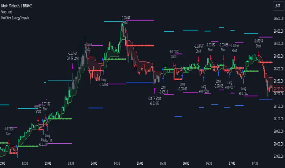
ProfitView Strategy TemplateHello traders,
This script took me a full week of coding/testing, sweat, and tears - and I’m too nice as I’m giving it for free to the community.
If you're tired of manual trading and looking for a solid strategy template to pair with your indicators, look no further.
This Pine Script v5 strategy template is engineered for maximum customization and risk management.
Best part?
This Pine Script v5 template facilitates the dynamic construction of ProfitView alerts, sparing users the time and effort of mastering the ProfitView syntax and manually creating alert commands.
This powerful tool gives much power to those who don't know how to code in Pinescript and want to automate their indicators' signals via the ProfitView Chrome extension.
IMPORTANT NOTES
ProfitView is a trading bot software that forwards TradingView alerts to your brokers (examples: Binance, Oanda, Coinbase, Bybit, etc.) for automating trading.
Many traders don't know how to dynamically create ProfitView-compatible alerts using the data from their TradingView scripts.
Traders using trading bots want their alerts to reflect the stop-loss/take-profit/trailing-stop/stop-loss to break options from your script and then create the orders accordingly.
This script showcases how to create ProfitView alerts dynamically.
TRADINGVIEW ALERTS
1) You'll have to create one alert per asset X timeframe = 1 chart.
Example: 1 alert for EUR/USD on the 5 minutes chart, 1 alert for EUR/USD on the 15-minute chart (assuming you want your bot to trade the EUR/USD on the 5 and 15-minute timeframes)
2) Select the Order fills and alert() function calls condition
3) For each alert, the alert message is pre-configured with the text below
{{strategy.order.alert_message}}
Please leave it as it is.
It's a TradingView native variable that will fetch the alert text messages built by the script.
4) ProfitView doesn't use webhook technology, so setting a webhook URL from the alerts notifications tab is unnecessary.
KEY FEATURES
I) Modular Indicator Connection
* plug your existing indicator into the template.
* Only two lines of code are needed for full compatibility.
Step 1: Create your connector
Adapt your indicator with only 2 lines of code and then connect it to this strategy template.
To do so:
1) Find in your indicator where the conditions print the long/buy and short/sell signals.
2) Create an additional plot as below
I'm giving an example with a Two moving averages cross.
Please replicate the same methodology for your indicator, whether a MACD , ZigZag, Pivots , higher-highs, lower-lows or whatever indicator with clear buy and sell conditions.
//@version=5
indicator("Supertrend", overlay = true, timeframe = "", timeframe_gaps = true)
atrPeriod = input.int(10, "ATR Length", minval = 1)
factor = input.float(3.0, "Factor", minval = 0.01, step = 0.01)
= ta.supertrend(factor, atrPeriod)
supertrend := barstate.isfirst ? na : supertrend
bodyMiddle = plot(barstate.isfirst ? na : (open + close) / 2, display = display.none)
upTrend = plot(direction < 0 ? supertrend : na, "Up Trend", color = color.green, style = plot.style_linebr)
downTrend = plot(direction < 0 ? na : supertrend, "Down Trend", color = color.red, style = plot.style_linebr)
fill(bodyMiddle, upTrend, color.new(color.green, 90), fillgaps = false)
fill(bodyMiddle, downTrend, color.new(color.red, 90), fillgaps = false)
buy = ta.crossunder(direction, 0)
sell = ta.crossunder(direction, 0)
//////// CONNECTOR SECTION ////////
Signal = buy ? 1 : sell ? -1 : 0
plot(Signal, title = "Signal", display = display.data_window)
//////// CONNECTOR SECTION ////////
Important Notes
🔥 The Strategy Template expects the value to be exactly 1 for the bullish signal and -1 for the bearish signal
Now, you can connect your indicator to the Strategy Template using the method below or that one.
Step 2: Connect the connector
1) Add your updated indicator to a TradingView chart
2) Add the Strategy Template as well to the SAME chart
3) Open the Strategy Template settings, and in the Data Source field, select your 🔌Connector🔌 (which comes from your indicator)
Note it doesn’t have to be named 🔌Connector🔌 - you can name it as you want - however, I recommend an explicit name you can easily remember.
From then, you should start seeing the signals and plenty of other stuff on your chart.
🔥 Note that whenever you update your indicator values, the strategy statistics and visuals on your chart will update in real-time
II) BOT Risk Management:
- Max Drawdown:
Mode: Select whether the max drawdown is calculated in percentage (%) or USD.
Value: If the max drawdown reaches this specified value, set a value to halt the bot.
- Max Consecutive Days:
Use Max Consecutive Days BOT Halt: Enable/Disable halting the bot if the max consecutive losing days value is reached.
- Max Consecutive Days: Set the maximum number of consecutive losing days allowed before halting the bot.
- Max Losing Streak:
Use Max Losing Streak: Enable/Disable a feature to prevent the bot from taking too many losses in a row.
- Max Losing Streak Length: Set the maximum length of a losing streak allowed.
Margin Call:
- Use Margin Call: Enable/Disable a feature to exit when a specified percentage away from a margin call to prevent it.
Margin Call (%): Set the percentage value to trigger this feature.
- Close BOT Total Loss:
Use Close BOT Total Loss: Enable/Disable a feature to close all trades and halt the bot if the total loss is reached.
- Total Loss ($): Set the total loss value in USD to trigger this feature.
Intraday BOT Risk Management:
- Intraday Losses:
Use Intraday Losses BOT Halt: Enable/Disable halting the bot on reaching specified intraday losses.
Mode: Select whether the intraday loss is calculated in percentage (%) or USD.
- Max Intraday Losses (%): Set the value for maximum intraday losses.
Limit Intraday Trades:
- Use Limit Intraday Trades: Enable/Disable a feature to limit the number of intraday trades.
- Max Intraday Trades: Set the maximum number of intraday trades allowed.
Restart Intraday EA:
- Use Restart Intraday EA: Enable/Disable a feature to restart the bot at the first bar of the next day if it has been stopped with an intraday risk management safeguard.
III) Order Types and Position Sizing
- Choose between market, limit, or stop orders.
- Set your position size directly in the template.
Please use the position size from the “Inputs” and not the “Properties” tab.
I know it's redundant. - the template needs this value from the "Inputs" tab to build the alerts, and the Backtester needs it from the "Properties" tab.
IV) Advanced Take-Profit and Stop-Loss Options
- Choose to set your SL/TP in either pips or percentages.
- Option for multiple take-profit levels and trailing stop losses.
- Move your stop loss to break even +/- offset in pips for “risk-free” trades.
V) Miscellaneous
Retry order openings if they fail.
Order Types:
Select and specify order type and price settings.
Position Size:
Define the type and size of positions.
Leverage:
Leverage settings, including margin type and hedge mode.
Session:
Limit trades to specific sessions.
Dates:
Limit trades to a specific date range.
Trades Direction:
Direction: Specify the market direction for opening positions.
VI) Notifications (Telegram/Discord/Email/IFTTT/Twilio/SMS)
Customize notifications sent to Telegram, Discord, Email, IFTTT, Twilio, and ProfitView Logger.
VII) Logger
The ProfitView commands are logged in the TradingView logger.
You'll find more information about it in this TradingView blog post .
WHY YOU MIGHT NEED THIS TEMPLATE
1) Transform your indicator into a ProfitView trading bot more easily than before
Connect your indicator to the template
Create your alerts
Set your EA settings
2) Save Time
Auto-generated alert messages for ProfitView.
I tested them all and checked with the support team what could/couldn’t be done.
3) Be in Control
Manage your trading risks with advanced features.
4) Customizable
Fits various trading styles and asset classes.
REQUIREMENTS
* Make sure you have your ProfitView account and do the settings correctly in your Chrome extension. If you don't know how to do it, read the documentation + ask for help in the ProfitView Discord support channel.
* If there is any issue with the template, ask me in the comments section - I’ll answer quickly.
BACKTEST RESULTS FROM THIS POST
1) I connected this strategy template to a dummy Supertrend script.
I could have selected any other indicator or concept for this script post.
I wanted to share an example of how you can quickly upgrade your strategy, making it compatible with ProfitView.
2) The backtest results aren't relevant for this educational script publication.
I used realistic backtesting data but didn't look too much into optimizing the results, as this isn't the point of why I'm publishing this script.
This strategy is a template to be connected to any indicator - the sky is the limit. :)
3) This template is made to take 1 trade per direction at any given time.
Pyramiding is set to 1 on TradingView.
The strategy default settings are:
* Initial Capital: 100000 USD
* Position Size: 1%
* Commission Percent: 0.075%
* Slippage: 1 tick
* No margin/leverage used
Best regards,
Dave
Adaptive Genesis Engine [AGE]ADAPTIVE GENESIS ENGINE (AGE)
Pure Signal Evolution Through Genetic Algorithms
Where Darwin Meets Technical Analysis
🧬 WHAT YOU'RE GETTING - THE PURE INDICATOR
This is a technical analysis indicator - it generates signals, visualizes probability, and shows you the evolutionary process in real-time. This is NOT a strategy with automatic execution - it's a sophisticated signal generation system that you control .
What This Indicator Does:
Generates Long/Short entry signals with probability scores (35-88% range)
Evolves a population of up to 12 competing strategies using genetic algorithms
Validates strategies through walk-forward optimization (train/test cycles)
Visualizes signal quality through premium gradient clouds and confidence halos
Displays comprehensive metrics via enhanced dashboard
Provides alerts for entries and exits
Works on any timeframe, any instrument, any broker
What This Indicator Does NOT Do:
Execute trades automatically
Manage positions or calculate position sizes
Place orders on your behalf
Make trading decisions for you
This is pure signal intelligence. AGE tells you when and how confident it is. You decide whether and how much to trade.
🔬 THE SCIENCE: GENETIC ALGORITHMS MEET TECHNICAL ANALYSIS
What Makes This Different - The Evolutionary Foundation
Most indicators are static - they use the same parameters forever, regardless of market conditions. AGE is alive . It maintains a population of competing strategies that evolve, adapt, and improve through natural selection principles:
Birth: New strategies spawn through crossover breeding (combining DNA from fit parents) plus random mutation for exploration
Life: Each strategy trades virtually via shadow portfolios, accumulating wins/losses, tracking drawdown, and building performance history
Selection: Strategies are ranked by comprehensive fitness scoring (win rate, expectancy, drawdown control, signal efficiency)
Death: Weak strategies are culled periodically, with elite performers (top 2 by default) protected from removal
Evolution: The gene pool continuously improves as successful traits propagate and unsuccessful ones die out
This is not curve-fitting. Each new strategy must prove itself on out-of-sample data through walk-forward validation before being trusted for live signals.
🧪 THE DNA: WHAT EVOLVES
Every strategy carries a 10-gene chromosome controlling how it interprets market data:
Signal Sensitivity Genes
Entropy Sensitivity (0.5-2.0): Weight given to market order/disorder calculations. Low values = conservative, require strong directional clarity. High values = aggressive, act on weaker order signals.
Momentum Sensitivity (0.5-2.0): Weight given to RSI/ROC/MACD composite. Controls responsiveness to momentum shifts vs. mean-reversion setups.
Structure Sensitivity (0.5-2.0): Weight given to support/resistance positioning. Determines how much price location within swing range matters.
Probability Adjustment Genes
Probability Boost (-0.10 to +0.10): Inherent bias toward aggressive (+) or conservative (-) entries. Acts as personality trait - some strategies naturally optimistic, others pessimistic.
Trend Strength Requirement (0.3-0.8): Minimum trend conviction needed before signaling. Higher values = only trades strong trends, lower values = acts in weak/sideways markets.
Volume Filter (0.5-1.5): Strictness of volume confirmation. Higher values = requires strong volume, lower values = volume less important.
Risk Management Genes
ATR Multiplier (1.5-4.0): Base volatility scaling for all price levels. Controls whether strategy uses tight or wide stops/targets relative to ATR.
Stop Multiplier (1.0-2.5): Stop loss tightness. Lower values = aggressive profit protection, higher values = more breathing room.
Target Multiplier (1.5-4.0): Profit target ambition. Lower values = quick scalping exits, higher values = swing trading holds.
Adaptation Gene
Regime Adaptation (0.0-1.0): How much strategy adjusts behavior based on detected market regime (trending/volatile/choppy). Higher values = more reactive to regime changes.
The Magic: AGE doesn't just try random combinations. Through tournament selection and fitness-weighted crossover, successful gene combinations spread through the population while unsuccessful ones fade away. Over 50-100 bars, you'll see the population converge toward genes that work for YOUR instrument and timeframe.
📊 THE SIGNAL ENGINE: THREE-LAYER SYNTHESIS
Before any strategy generates a signal, AGE calculates probability through multi-indicator confluence:
Layer 1 - Market Entropy (Information Theory)
Measures whether price movements exhibit directional order or random walk characteristics:
The Math:
Shannon Entropy = -Σ(p × log(p))
Market Order = 1 - (Entropy / 0.693)
What It Means:
High entropy = choppy, random market → low confidence signals
Low entropy = directional market → high confidence signals
Direction determined by up-move vs down-move dominance over lookback period (default: 20 bars)
Signal Output: -1.0 to +1.0 (bearish order to bullish order)
Layer 2 - Momentum Synthesis
Combines three momentum indicators into single composite score:
Components:
RSI (40% weight): Normalized to -1/+1 scale using (RSI-50)/50
Rate of Change (30% weight): Percentage change over lookback (default: 14 bars), clamped to ±1
MACD Histogram (30% weight): Fast(12) - Slow(26), normalized by ATR
Why This Matters: RSI catches mean-reversion opportunities, ROC catches raw momentum, MACD catches momentum divergence. Weighting favors RSI for reliability while keeping other perspectives.
Signal Output: -1.0 to +1.0 (strong bearish to strong bullish)
Layer 3 - Structure Analysis
Evaluates price position within swing range (default: 50-bar lookback):
Position Classification:
Bottom 20% of range = Support Zone → bullish bounce potential
Top 20% of range = Resistance Zone → bearish rejection potential
Middle 60% = Neutral Zone → breakout/breakdown monitoring
Signal Logic:
At support + bullish candle = +0.7 (strong buy setup)
At resistance + bearish candle = -0.7 (strong sell setup)
Breaking above range highs = +0.5 (breakout confirmation)
Breaking below range lows = -0.5 (breakdown confirmation)
Consolidation within range = ±0.3 (weak directional bias)
Signal Output: -1.0 to +1.0 (bearish structure to bullish structure)
Confluence Voting System
Each layer casts a vote (Long/Short/Neutral). The system requires minimum 2-of-3 agreement (configurable 1-3) before generating a signal:
Examples:
Entropy: Bullish, Momentum: Bullish, Structure: Neutral → Signal generated (2 long votes)
Entropy: Bearish, Momentum: Neutral, Structure: Neutral → No signal (only 1 short vote)
All three bullish → Signal generated with +5% probability bonus
This is the key to quality. Single indicators give too many false signals. Triple confirmation dramatically improves accuracy.
📈 PROBABILITY CALCULATION: HOW CONFIDENCE IS MEASURED
Base Probability:
Raw_Prob = 50% + (Average_Signal_Strength × 25%)
Then AGE applies strategic adjustments:
Trend Alignment:
Signal with trend: +4%
Signal against strong trend: -8%
Weak/no trend: no adjustment
Regime Adaptation:
Trending market (efficiency >50%, moderate vol): +3%
Volatile market (vol ratio >1.5x): -5%
Choppy market (low efficiency): -2%
Volume Confirmation:
Volume > 70% of 20-bar SMA: no change
Volume below threshold: -3%
Volatility State (DVS Ratio):
High vol (>1.8x baseline): -4% (reduce confidence in chaos)
Low vol (<0.7x baseline): -2% (markets can whipsaw in compression)
Moderate elevated vol (1.0-1.3x): +2% (trending conditions emerging)
Confluence Bonus:
All 3 indicators agree: +5%
2 of 3 agree: +2%
Strategy Gene Adjustment:
Probability Boost gene: -10% to +10%
Regime Adaptation gene: scales regime adjustments by 0-100%
Final Probability: Clamped between 35% (minimum) and 88% (maximum)
Why These Ranges?
Below 35% = too uncertain, better not to signal
Above 88% = unrealistic, creates overconfidence
Sweet spot: 65-80% for quality entries
🔄 THE SHADOW PORTFOLIO SYSTEM: HOW STRATEGIES COMPETE
Each active strategy maintains a virtual trading account that executes in parallel with real-time data:
Shadow Trading Mechanics
Entry Logic:
Calculate signal direction, probability, and confluence using strategy's unique DNA
Check if signal meets quality gate:
Probability ≥ configured minimum threshold (default: 65%)
Confluence ≥ configured minimum (default: 2 of 3)
Direction is not zero (must be long or short, not neutral)
Verify signal persistence:
Base requirement: 2 bars (configurable 1-5)
Adapts based on probability: high-prob signals (75%+) enter 1 bar faster, low-prob signals need 1 bar more
Adjusts for regime: trending markets reduce persistence by 1, volatile markets add 1
Apply additional filters:
Trend strength must exceed strategy's requirement gene
Regime filter: if volatile market detected, probability must be 72%+ to override
Volume confirmation required (volume > 70% of average)
If all conditions met for required persistence bars, enter shadow position at current close price
Position Management:
Entry Price: Recorded at close of entry bar
Stop Loss: ATR-based distance = ATR × ATR_Mult (gene) × Stop_Mult (gene) × DVS_Ratio
Take Profit: ATR-based distance = ATR × ATR_Mult (gene) × Target_Mult (gene) × DVS_Ratio
Position: +1 (long) or -1 (short), only one at a time per strategy
Exit Logic:
Check if price hit stop (on low) or target (on high) on current bar
Record trade outcome in R-multiples (profit/loss normalized by ATR)
Update performance metrics:
Total trades counter incremented
Wins counter (if profit > 0)
Cumulative P&L updated
Peak equity tracked (for drawdown calculation)
Maximum drawdown from peak recorded
Enter cooldown period (default: 8 bars, configurable 3-20) before next entry allowed
Reset signal age counter to zero
Walk-Forward Tracking:
During position lifecycle, trades are categorized:
Training Phase (first 250 bars): Trade counted toward training metrics
Testing Phase (next 75 bars): Trade counted toward testing metrics (out-of-sample)
Live Phase (after WFO period): Trade counted toward overall metrics
Why Shadow Portfolios?
No lookahead bias (uses only data available at the bar)
Realistic execution simulation (entry on close, stop/target checks on high/low)
Independent performance tracking for true fitness comparison
Allows safe experimentation without risking capital
Each strategy learns from its own experience
🏆 FITNESS SCORING: HOW STRATEGIES ARE RANKED
Fitness is not just win rate. AGE uses a comprehensive multi-factor scoring system:
Core Metrics (Minimum 3 trades required)
Win Rate (30% of fitness):
WinRate = Wins / TotalTrades
Normalized directly (0.0-1.0 scale)
Total P&L (30% of fitness):
Normalized_PnL = (PnL + 300) / 600
Clamped 0.0-1.0. Assumes P&L range of -300R to +300R for normalization scale.
Expectancy (25% of fitness):
Expectancy = Total_PnL / Total_Trades
Normalized_Expectancy = (Expectancy + 30) / 60
Clamped 0.0-1.0. Rewards consistency of profit per trade.
Drawdown Control (15% of fitness):
Normalized_DD = 1 - (Max_Drawdown / 15)
Clamped 0.0-1.0. Penalizes strategies that suffer large equity retracements from peak.
Sample Size Adjustment
Quality Factor:
<50 trades: 1.0 (full weight, small sample)
50-100 trades: 0.95 (slight penalty for medium sample)
100 trades: 0.85 (larger penalty for large sample)
Why penalize more trades? Prevents strategies from gaming the system by taking hundreds of tiny trades to inflate statistics. Favors quality over quantity.
Bonus Adjustments
Walk-Forward Validation Bonus:
if (WFO_Validated):
Fitness += (WFO_Efficiency - 0.5) × 0.1
Strategies proven on out-of-sample data receive up to +10% fitness boost based on test/train efficiency ratio.
Signal Efficiency Bonus (if diagnostics enabled):
if (Signals_Evaluated > 10):
Pass_Rate = Signals_Passed / Signals_Evaluated
Fitness += (Pass_Rate - 0.1) × 0.05
Rewards strategies that generate high-quality signals passing the quality gate, not just profitable trades.
Final Fitness: Clamped at 0.0 minimum (prevents negative fitness values)
Result: Elite strategies typically achieve 0.50-0.75 fitness. Anything above 0.60 is excellent. Below 0.30 is prime candidate for culling.
🔬 WALK-FORWARD OPTIMIZATION: ANTI-OVERFITTING PROTECTION
This is what separates AGE from curve-fitted garbage indicators.
The Three-Phase Process
Every new strategy undergoes a rigorous validation lifecycle:
Phase 1 - Training Window (First 250 bars, configurable 100-500):
Strategy trades normally via shadow portfolio
All trades count toward training performance metrics
System learns which gene combinations produce profitable patterns
Tracks independently: Training_Trades, Training_Wins, Training_PnL
Phase 2 - Testing Window (Next 75 bars, configurable 30-200):
Strategy continues trading without any parameter changes
Trades now count toward testing performance metrics (separate tracking)
This is out-of-sample data - strategy has never seen these bars during "optimization"
Tracks independently: Testing_Trades, Testing_Wins, Testing_PnL
Phase 3 - Validation Check:
Minimum_Trades = 5 (configurable 3-15)
IF (Train_Trades >= Minimum AND Test_Trades >= Minimum):
WR_Efficiency = Test_WinRate / Train_WinRate
Expectancy_Efficiency = Test_Expectancy / Train_Expectancy
WFO_Efficiency = (WR_Efficiency + Expectancy_Efficiency) / 2
IF (WFO_Efficiency >= 0.55): // configurable 0.3-0.9
Strategy.Validated = TRUE
Strategy receives fitness bonus
ELSE:
Strategy receives 30% fitness penalty
ELSE:
Validation deferred (insufficient trades in one or both periods)
What Validation Means
Validated Strategy (Green "✓ VAL" in dashboard):
Performed at least 55% as well on unseen data compared to training data
Gets fitness bonus: +(efficiency - 0.5) × 0.1
Receives priority during tournament selection for breeding
More likely to be chosen as active trading strategy
Unvalidated Strategy (Orange "○ TRAIN" in dashboard):
Failed to maintain performance on test data (likely curve-fitted to training period)
Receives 30% fitness penalty (0.7x multiplier)
Makes strategy prime candidate for culling
Can still trade but with lower selection probability
Insufficient Data (continues collecting):
Hasn't completed both training and testing periods yet
OR hasn't achieved minimum trade count in both periods
Validation check deferred until requirements met
Why 55% Efficiency Threshold?
If a strategy earned 10R during training but only 5.5R during testing, it still proved an edge exists beyond random luck. Requiring 100% efficiency would be unrealistic - market conditions change between periods. But requiring >50% ensures the strategy didn't completely degrade on fresh data.
The Protection: Strategies that work great on historical data but fail on new data are automatically identified and penalized. This prevents the population from being polluted by overfitted strategies that would fail in live trading.
🌊 DYNAMIC VOLATILITY SCALING (DVS): ADAPTIVE STOP/TARGET PLACEMENT
AGE doesn't use fixed stop distances. It adapts to current volatility conditions in real-time.
Four Volatility Measurement Methods
1. ATR Ratio (Simple Method):
Current_Vol = ATR(14) / Close
Baseline_Vol = SMA(Current_Vol, 100)
Ratio = Current_Vol / Baseline_Vol
Basic comparison of current ATR to 100-bar moving average baseline.
2. Parkinson (High-Low Range Based):
For each bar: HL = log(High / Low)
Parkinson_Vol = sqrt(Σ(HL²) / (4 × Period × log(2)))
More stable than close-to-close volatility. Captures intraday range expansion without overnight gap noise.
3. Garman-Klass (OHLC Based):
HL_Term = 0.5 × ²
CO_Term = (2×log(2) - 1) × ²
GK_Vol = sqrt(Σ(HL_Term - CO_Term) / Period)
Most sophisticated estimator. Incorporates all four price points (open, high, low, close) plus gap information.
4. Ensemble Method (Default - Median of All Three):
Ratio_1 = ATR_Current / ATR_Baseline
Ratio_2 = Parkinson_Current / Parkinson_Baseline
Ratio_3 = GK_Current / GK_Baseline
DVS_Ratio = Median(Ratio_1, Ratio_2, Ratio_3)
Why Ensemble?
Takes median to avoid outliers and false spikes
If ATR jumps but range-based methods stay calm, median prevents overreaction
If one method fails, other two compensate
Most robust approach across different market conditions
Sensitivity Scaling
Scaled_Ratio = (Raw_Ratio) ^ Sensitivity
Sensitivity 0.3: Cube root - heavily dampens volatility impact
Sensitivity 0.5: Square root - moderate dampening
Sensitivity 0.7 (Default): Balanced response to volatility changes
Sensitivity 1.0: Linear - full 1:1 volatility impact
Sensitivity 1.5: Exponential - amplified response to volatility spikes
Safety Clamps: Final DVS Ratio always clamped between 0.5x and 2.5x baseline to prevent extreme position sizing or stop placement errors.
How DVS Affects Shadow Trading
Every strategy's stop and target distances are multiplied by the current DVS ratio:
Stop Loss Distance:
Stop_Distance = ATR × ATR_Mult (gene) × Stop_Mult (gene) × DVS_Ratio
Take Profit Distance:
Target_Distance = ATR × ATR_Mult (gene) × Target_Mult (gene) × DVS_Ratio
Example Scenario:
ATR = 10 points
Strategy's ATR_Mult gene = 2.5
Strategy's Stop_Mult gene = 1.5
Strategy's Target_Mult gene = 2.5
DVS_Ratio = 1.4 (40% above baseline volatility - market heating up)
Stop = 10 × 2.5 × 1.5 × 1.4 = 52.5 points (vs. 37.5 in normal vol)
Target = 10 × 2.5 × 2.5 × 1.4 = 87.5 points (vs. 62.5 in normal vol)
Result:
During volatility spikes: Stops automatically widen to avoid noise-based exits, targets extend for bigger moves
During calm periods: Stops tighten for better risk/reward, targets compress for realistic profit-taking
Strategies adapt risk management to match current market behavior
🧬 THE EVOLUTIONARY CYCLE: SPAWN, COMPETE, CULL
Initialization (Bar 1)
AGE begins with 4 seed strategies (if evolution enabled):
Seed Strategy #0 (Balanced):
All sensitivities at 1.0 (neutral)
Zero probability boost
Moderate trend requirement (0.4)
Standard ATR/stop/target multiples (2.5/1.5/2.5)
Mid-level regime adaptation (0.5)
Seed Strategy #1 (Momentum-Focused):
Lower entropy sensitivity (0.7), higher momentum (1.5)
Slight probability boost (+0.03)
Higher trend requirement (0.5)
Tighter stops (1.3), wider targets (3.0)
Seed Strategy #2 (Entropy-Driven):
Higher entropy sensitivity (1.5), lower momentum (0.8)
Slight probability penalty (-0.02)
More trend tolerant (0.6)
Wider stops (1.8), standard targets (2.5)
Seed Strategy #3 (Structure-Based):
Balanced entropy/momentum (0.8/0.9), high structure (1.4)
Slight probability boost (+0.02)
Lower trend requirement (0.35)
Moderate risk parameters (1.6/2.8)
All seeds start with WFO validation bypassed if WFO is disabled, or must validate if enabled.
Spawning New Strategies
Timing (Adaptive):
Historical phase: Every 30 bars (configurable 10-100)
Live phase: Every 200 bars (configurable 100-500)
Automatically switches to live timing when barstate.isrealtime triggers
Conditions:
Current population < max population limit (default: 8, configurable 4-12)
At least 2 active strategies exist (need parents)
Available slot in population array
Selection Process:
Run tournament selection 3 times with different seeds
Each tournament: randomly sample active strategies, pick highest fitness
Best from 3 tournaments becomes Parent 1
Repeat independently for Parent 2
Ensures fit parents but maintains diversity
Crossover Breeding:
For each of 10 genes:
Parent1_Fitness = fitness
Parent2_Fitness = fitness
Weight1 = Parent1_Fitness / (Parent1_Fitness + Parent2_Fitness)
Gene1 = parent1's value
Gene2 = parent2's value
Child_Gene = Weight1 × Gene1 + (1 - Weight1) × Gene2
Fitness-weighted crossover ensures fitter parent contributes more genetic material.
Mutation:
For each gene in child:
IF (random < mutation_rate):
Gene_Range = GENE_MAX - GENE_MIN
Noise = (random - 0.5) × 2 × mutation_strength × Gene_Range
Mutated_Gene = Clamp(Child_Gene + Noise, GENE_MIN, GENE_MAX)
Historical mutation rate: 20% (aggressive exploration)
Live mutation rate: 8% (conservative stability)
Mutation strength: 12% of gene range (configurable 5-25%)
Initialization of New Strategy:
Unique ID assigned (total_spawned counter)
Parent ID recorded
Generation = max(parent generations) + 1
Birth bar recorded (for age tracking)
All performance metrics zeroed
Shadow portfolio reset
WFO validation flag set to false (must prove itself)
Result: New strategy with hybrid DNA enters population, begins trading in next bar.
Competition (Every Bar)
All active strategies:
Calculate their signal based on unique DNA
Check quality gate with their thresholds
Manage shadow positions (entries/exits)
Update performance metrics
Recalculate fitness score
Track WFO validation progress
Strategies compete indirectly through fitness ranking - no direct interaction.
Culling Weak Strategies
Timing (Adaptive):
Historical phase: Every 60 bars (configurable 20-200, should be 2x spawn interval)
Live phase: Every 400 bars (configurable 200-1000, should be 2x spawn interval)
Minimum Adaptation Score (MAS):
Initial MAS = 0.10
MAS decays: MAS × 0.995 every cull cycle
Minimum MAS = 0.03 (floor)
MAS represents the "survival threshold" - strategies below this fitness level are vulnerable.
Culling Conditions (ALL must be true):
Population > minimum population (default: 3, configurable 2-4)
At least one strategy has fitness < MAS
Strategy's age > culling interval (prevents premature culling of new strategies)
Strategy is not in top N elite (default: 2, configurable 1-3)
Culling Process:
Find worst strategy:
For each active strategy:
IF (age > cull_interval):
Fitness = base_fitness
IF (not WFO_validated AND WFO_enabled):
Fitness × 0.7 // 30% penalty for unvalidated
IF (Fitness < MAS AND Fitness < worst_fitness_found):
worst_strategy = this_strategy
worst_fitness = Fitness
IF (worst_strategy found):
Count elite strategies with fitness > worst_fitness
IF (elite_count >= elite_preservation_count):
Deactivate worst_strategy (set active flag = false)
Increment total_culled counter
Elite Protection:
Even if a strategy's fitness falls below MAS, it survives if fewer than N strategies are better. This prevents culling when population is generally weak.
Result: Weak strategies removed from population, freeing slots for new spawns. Gene pool improves over time.
Selection for Display (Every Bar)
AGE chooses one strategy to display signals:
Best fitness = -1
Selected = none
For each active strategy:
Fitness = base_fitness
IF (WFO_validated):
Fitness × 1.3 // 30% bonus for validated strategies
IF (Fitness > best_fitness):
best_fitness = Fitness
selected_strategy = this_strategy
Display selected strategy's signals on chart
Result: Only the highest-fitness (optionally validated-boosted) strategy's signals appear as chart markers. Other strategies trade invisibly in shadow portfolios.
🎨 PREMIUM VISUALIZATION SYSTEM
AGE includes sophisticated visual feedback that standard indicators lack:
1. Gradient Probability Cloud (Optional, Default: ON)
Multi-layer gradient showing signal buildup 2-3 bars before entry:
Activation Conditions:
Signal persistence > 0 (same directional signal held for multiple bars)
Signal probability ≥ minimum threshold (65% by default)
Signal hasn't yet executed (still in "forming" state)
Visual Construction:
7 gradient layers by default (configurable 3-15)
Each layer is a line-fill pair (top line, bottom line, filled between)
Layer spacing: 0.3 to 1.0 × ATR above/below price
Outer layers = faint, inner layers = bright
Color transitions from base to intense based on layer position
Transparency scales with probability (high prob = more opaque)
Color Selection:
Long signals: Gradient from theme.gradient_bull_mid to theme.gradient_bull_strong
Short signals: Gradient from theme.gradient_bear_mid to theme.gradient_bear_strong
Base transparency: 92%, reduces by up to 8% for high-probability setups
Dynamic Behavior:
Cloud grows/shrinks as signal persistence increases/decreases
Redraws every bar while signal is forming
Disappears when signal executes or invalidates
Performance Note: Computationally expensive due to linefill objects. Disable or reduce layers if chart performance degrades.
2. Population Fitness Ribbon (Optional, Default: ON)
Histogram showing fitness distribution across active strategies:
Activation: Only draws on last bar (barstate.islast) to avoid historical clutter
Visual Construction:
10 histogram layers by default (configurable 5-20)
Plots 50 bars back from current bar
Positioned below price at: lowest_low(100) - 1.5×ATR (doesn't interfere with price action)
Each layer represents a fitness threshold (evenly spaced min to max fitness)
Layer Logic:
For layer_num from 0 to ribbon_layers:
Fitness_threshold = min_fitness + (max_fitness - min_fitness) × (layer / layers)
Count strategies with fitness ≥ threshold
Height = ATR × 0.15 × (count / total_active)
Y_position = base_level + ATR × 0.2 × layer
Color = Gradient from weak to strong based on layer position
Line_width = Scaled by height (taller = thicker)
Visual Feedback:
Tall, bright ribbon = healthy population, many fit strategies at high fitness levels
Short, dim ribbon = weak population, few strategies achieving good fitness
Ribbon compression (layers close together) = population converging to similar fitness
Ribbon spread = diverse fitness range, active selection pressure
Use Case: Quick visual health check without opening dashboard. Ribbon growing upward over time = population improving.
3. Confidence Halo (Optional, Default: ON)
Circular polyline around entry signals showing probability strength:
Activation: Draws when new position opens (shadow_position changes from 0 to ±1)
Visual Construction:
20-segment polyline forming approximate circle
Center: Low - 0.5×ATR (long) or High + 0.5×ATR (short)
Radius: 0.3×ATR (low confidence) to 1.0×ATR (elite confidence)
Scales with: (probability - min_probability) / (1.0 - min_probability)
Color Coding:
Elite (85%+): Cyan (theme.conf_elite), large radius, minimal transparency (40%)
Strong (75-85%): Strong green (theme.conf_strong), medium radius, moderate transparency (50%)
Good (65-75%): Good green (theme.conf_good), smaller radius, more transparent (60%)
Moderate (<65%): Moderate green (theme.conf_moderate), tiny radius, very transparent (70%)
Technical Detail:
Uses chart.point array with index-based positioning
5-bar horizontal spread for circular appearance (±5 bars from entry)
Curved=false (Pine Script polyline limitation)
Fill color matches line color but more transparent (88% vs line's transparency)
Purpose: Instant visual probability assessment. No need to check dashboard - halo size/brightness tells the story.
4. Evolution Event Markers (Optional, Default: ON)
Visual indicators of genetic algorithm activity:
Spawn Markers (Diamond, Cyan):
Plots when total_spawned increases on current bar
Location: bottom of chart (location.bottom)
Color: theme.spawn_marker (cyan/bright blue)
Size: tiny
Indicates new strategy just entered population
Cull Markers (X-Cross, Red):
Plots when total_culled increases on current bar
Location: bottom of chart (location.bottom)
Color: theme.cull_marker (red/pink)
Size: tiny
Indicates weak strategy just removed from population
What It Tells You:
Frequent spawning early = population building, active exploration
Frequent culling early = high selection pressure, weak strategies dying fast
Balanced spawn/cull = healthy evolutionary churn
No markers for long periods = stable population (evolution plateaued or optimal genes found)
5. Entry/Exit Markers
Clear visual signals for selected strategy's trades:
Long Entry (Triangle Up, Green):
Plots when selected strategy opens long position (position changes 0 → +1)
Location: below bar (location.belowbar)
Color: theme.long_primary (green/cyan depending on theme)
Transparency: Scales with probability:
Elite (85%+): 0% (fully opaque)
Strong (75-85%): 10%
Good (65-75%): 20%
Acceptable (55-65%): 35%
Size: small
Short Entry (Triangle Down, Red):
Plots when selected strategy opens short position (position changes 0 → -1)
Location: above bar (location.abovebar)
Color: theme.short_primary (red/pink depending on theme)
Transparency: Same scaling as long entries
Size: small
Exit (X-Cross, Orange):
Plots when selected strategy closes position (position changes ±1 → 0)
Location: absolute (at actual exit price if stop/target lines enabled)
Color: theme.exit_color (orange/yellow depending on theme)
Transparency: 0% (fully opaque)
Size: tiny
Result: Clean, probability-scaled markers that don't clutter chart but convey essential information.
6. Stop Loss & Take Profit Lines (Optional, Default: ON)
Visual representation of shadow portfolio risk levels:
Stop Loss Line:
Plots when selected strategy has active position
Level: shadow_stop value from selected strategy
Color: theme.short_primary with 60% transparency (red/pink, subtle)
Width: 2
Style: plot.style_linebr (breaks when no position)
Take Profit Line:
Plots when selected strategy has active position
Level: shadow_target value from selected strategy
Color: theme.long_primary with 60% transparency (green, subtle)
Width: 2
Style: plot.style_linebr (breaks when no position)
Purpose:
Shows where shadow portfolio would exit for stop/target
Helps visualize strategy's risk/reward ratio
Useful for manual traders to set similar levels
Disable for cleaner chart (recommended for presentations)
7. Dynamic Trend EMA
Gradient-colored trend line that visualizes trend strength:
Calculation:
EMA(close, trend_length) - default 50 period (configurable 20-100)
Slope calculated over 10 bars: (current_ema - ema ) / ema × 100
Color Logic:
Trend_direction:
Slope > 0.1% = Bullish (1)
Slope < -0.1% = Bearish (-1)
Otherwise = Neutral (0)
Trend_strength = abs(slope)
Color = Gradient between:
- Neutral color (gray/purple)
- Strong bullish (bright green) if direction = 1
- Strong bearish (bright red) if direction = -1
Gradient factor = trend_strength (0 to 1+ scale)
Visual Behavior:
Faint gray/purple = weak/no trend (choppy conditions)
Light green/red = emerging trend (low strength)
Bright green/red = strong trend (high conviction)
Color intensity = trend strength magnitude
Transparency: 50% (subtle, doesn't overpower price action)
Purpose: Subconscious awareness of trend state without checking dashboard or indicators.
8. Regime Background Tinting (Subtle)
Ultra-low opacity background color indicating detected market regime:
Regime Detection:
Efficiency = directional_movement / total_range (over trend_length bars)
Vol_ratio = current_volatility / average_volatility
IF (efficiency > 0.5 AND vol_ratio < 1.3):
Regime = Trending (1)
ELSE IF (vol_ratio > 1.5):
Regime = Volatile (2)
ELSE:
Regime = Choppy (0)
Background Colors:
Trending: theme.regime_trending (dark green, 92-93% transparency)
Volatile: theme.regime_volatile (dark red, 93% transparency)
Choppy: No tint (normal background)
Purpose:
Subliminal regime awareness
Helps explain why signals are/aren't generating
Trending = ideal conditions for AGE
Volatile = fewer signals, higher thresholds applied
Choppy = mixed signals, lower confidence
Important: Extremely subtle by design. Not meant to be obvious, just subconscious context.
📊 ENHANCED DASHBOARD
Comprehensive real-time metrics in single organized panel (top-right position):
Dashboard Structure (5 columns × 14 rows)
Header Row:
Column 0: "🧬 AGE PRO" + phase indicator (🔴 LIVE or ⏪ HIST)
Column 1: "POPULATION"
Column 2: "PERFORMANCE"
Column 3: "CURRENT SIGNAL"
Column 4: "ACTIVE STRATEGY"
Column 0: Market State
Regime (📈 TREND / 🌊 CHAOS / ➖ CHOP)
DVS Ratio (current volatility scaling factor, format: #.##)
Trend Direction (▲ BULL / ▼ BEAR / ➖ FLAT with color coding)
Trend Strength (0-100 scale, format: #.##)
Column 1: Population Metrics
Active strategies (count / max_population)
Validated strategies (WFO passed / active total)
Current generation number
Total spawned (all-time strategy births)
Total culled (all-time strategy deaths)
Column 2: Aggregate Performance
Total trades across all active strategies
Aggregate win rate (%) - color-coded:
Green (>55%)
Orange (45-55%)
Red (<45%)
Total P&L in R-multiples - color-coded by positive/negative
Best fitness score in population (format: #.###)
MAS - Minimum Adaptation Score (cull threshold, format: #.###)
Column 3: Current Signal Status
Status indicator:
"▲ LONG" (green) if selected strategy in long position
"▼ SHORT" (red) if selected strategy in short position
"⏳ FORMING" (orange) if signal persisting but not yet executed
"○ WAITING" (gray) if no active signal
Confidence percentage (0-100%, format: #.#%)
Quality assessment:
"🔥 ELITE" (cyan) for 85%+ probability
"✓ STRONG" (bright green) for 75-85%
"○ GOOD" (green) for 65-75%
"- LOW" (dim) for <65%
Confluence score (X/3 format)
Signal age:
"X bars" if signal forming
"IN TRADE" if position active
"---" if no signal
Column 4: Selected Strategy Details
Strategy ID number (#X format)
Validation status:
"✓ VAL" (green) if WFO validated
"○ TRAIN" (orange) if still in training/testing phase
Generation number (GX format)
Personal fitness score (format: #.### with color coding)
Trade count
P&L and win rate (format: #.#R (##%) with color coding)
Color Scheme:
Panel background: theme.panel_bg (dark, low opacity)
Panel headers: theme.panel_header (slightly lighter)
Primary text: theme.text_primary (bright, high contrast)
Secondary text: theme.text_secondary (dim, lower contrast)
Positive metrics: theme.metric_positive (green)
Warning metrics: theme.metric_warning (orange)
Negative metrics: theme.metric_negative (red)
Special markers: theme.validated_marker, theme.spawn_marker
Update Frequency: Only on barstate.islast (current bar) to minimize CPU usage
Purpose:
Quick overview of entire system state
No need to check multiple indicators
Trading decisions informed by population health, regime state, and signal quality
Transparency into what AGE is thinking
🔍 DIAGNOSTICS PANEL (Optional, Default: OFF)
Detailed signal quality tracking for optimization and debugging:
Panel Structure (3 columns × 8 rows)
Position: Bottom-right corner (doesn't interfere with main dashboard)
Header Row:
Column 0: "🔍 DIAGNOSTICS"
Column 1: "COUNT"
Column 2: "%"
Metrics Tracked (for selected strategy only):
Total Evaluated:
Every signal that passed initial calculation (direction ≠ 0)
Represents total opportunities considered
✓ Passed:
Signals that passed quality gate and executed
Green color coding
Percentage of evaluated signals
Rejection Breakdown:
⨯ Probability:
Rejected because probability < minimum threshold
Most common rejection reason typically
⨯ Confluence:
Rejected because confluence < minimum required (e.g., only 1 of 3 indicators agreed)
⨯ Trend:
Rejected because signal opposed strong trend
Indicates counter-trend protection working
⨯ Regime:
Rejected because volatile regime detected and probability wasn't high enough to override
Shows regime filter in action
⨯ Volume:
Rejected because volume < 70% of 20-bar average
Indicates volume confirmation requirement
Color Coding:
Passed count: Green (success metric)
Rejection counts: Red (failure metrics)
Percentages: Gray (neutral, informational)
Performance Cost: Slight CPU overhead for tracking counters. Disable when not actively optimizing settings.
How to Use Diagnostics
Scenario 1: Too Few Signals
Evaluated: 200
Passed: 10 (5%)
⨯ Probability: 120 (60%)
⨯ Confluence: 40 (20%)
⨯ Others: 30 (15%)
Diagnosis: Probability threshold too high for this strategy's DNA.
Solution: Lower min probability from 65% to 60%, or allow strategy more time to evolve better DNA.
Scenario 2: Too Many False Signals
Evaluated: 200
Passed: 80 (40%)
Strategy win rate: 45%
Diagnosis: Quality gate too loose, letting low-quality signals through.
Solution: Raise min probability to 70%, or increase min confluence to 3 (all indicators must agree).
Scenario 3: Regime-Specific Issues
⨯ Regime: 90 (45% of rejections)
Diagnosis: Frequent volatile regime detection blocking otherwise good signals.
Solution: Either accept fewer trades during chaos (recommended), or disable regime filter if you want signals regardless of market state.
Optimization Workflow:
Enable diagnostics
Run 200+ bars
Analyze rejection patterns
Adjust settings based on data
Re-run and compare pass rate
Disable diagnostics when satisfied
⚙️ CONFIGURATION GUIDE
🧬 Evolution Engine Settings
Enable AGE Evolution (Default: ON):
ON: Full genetic algorithm (recommended for best results)
OFF: Uses only 4 seed strategies, no spawning/culling (static population for comparison testing)
Max Population (4-12, Default: 8):
Higher = more diversity, more exploration, slower performance
Lower = faster computation, less exploration, risk of premature convergence
Sweet spot: 6-8 for most use cases
4 = minimum for meaningful evolution
12 = maximum before diminishing returns
Min Population (2-4, Default: 3):
Safety floor - system never culls below this count
Prevents population extinction during harsh selection
Should be at least half of max population
Elite Preservation (1-3, Default: 2):
Top N performers completely immune to culling
Ensures best genes always survive
1 = minimal protection, aggressive selection
2 = balanced (recommended)
3 = conservative, slower gene pool turnover
Historical: Spawn Interval (10-100, Default: 30):
Bars between spawning new strategies during historical data
Lower = faster evolution, more exploration
Higher = slower evolution, more evaluation time per strategy
30 bars = ~1-2 hours on 15min chart
Historical: Cull Interval (20-200, Default: 60):
Bars between culling weak strategies during historical data
Should be 2x spawn interval for balanced churn
Lower = aggressive selection pressure
Higher = patient evaluation
Live: Spawn Interval (100-500, Default: 200):
Bars between spawning during live trading
Much slower than historical for stability
Prevents population chaos during live trading
200 bars = ~1.5 trading days on 15min chart
Live: Cull Interval (200-1000, Default: 400):
Bars between culling during live trading
Should be 2x live spawn interval
Conservative removal during live trading
Historical: Mutation Rate (0.05-0.40, Default: 0.20):
Probability each gene mutates during breeding (20% = 2 out of 10 genes on average)
Higher = more exploration, slower convergence
Lower = more exploitation, faster convergence but risk of local optima
20% balances exploration vs exploitation
Live: Mutation Rate (0.02-0.20, Default: 0.08):
Mutation rate during live trading
Much lower for stability (don't want population to suddenly degrade)
8% = mostly inherits parent genes with small tweaks
Mutation Strength (0.05-0.25, Default: 0.12):
How much genes change when mutated (% of gene's total range)
0.05 = tiny nudges (fine-tuning)
0.12 = moderate jumps (recommended)
0.25 = large leaps (aggressive exploration)
Example: If gene range is 0.5-2.0, 12% strength = ±0.18 possible change
📈 Signal Quality Settings
Min Signal Probability (0.55-0.80, Default: 0.65):
Quality gate threshold - signals below this never generate
0.55-0.60 = More signals, accept lower confidence (higher risk)
0.65 = Institutional-grade balance (recommended)
0.70-0.75 = Fewer but higher-quality signals (conservative)
0.80+ = Very selective, very few signals (ultra-conservative)
Min Confluence Score (1-3, Default: 2):
Required indicator agreement before signal generates
1 = Any single indicator can trigger (not recommended - too many false signals)
2 = Requires 2 of 3 indicators agree (RECOMMENDED for balance)
3 = All 3 must agree (very selective, few signals, high quality)
Base Persistence Bars (1-5, Default: 2):
Base bars signal must persist before entry
System adapts automatically:
High probability signals (75%+) enter 1 bar faster
Low probability signals (<68%) need 1 bar more
Trending regime: -1 bar (faster entries)
Volatile regime: +1 bar (more confirmation)
1 = Immediate entry after quality gate (responsive but prone to whipsaw)
2 = Balanced confirmation (recommended)
3-5 = Patient confirmation (slower but more reliable)
Cooldown After Trade (3-20, Default: 8):
Bars to wait after exit before next entry allowed
Prevents overtrading and revenge trading
3 = Minimal cooldown (active trading)
8 = Balanced (recommended)
15-20 = Conservative (position trading)
Entropy Length (10-50, Default: 20):
Lookback period for market order/disorder calculation
Lower = more responsive to regime changes (noisy)
Higher = more stable regime detection (laggy)
20 = works across most timeframes
Momentum Length (5-30, Default: 14):
Period for RSI/ROC calculations
14 = standard (RSI default)
Lower = more signals, less reliable
Higher = fewer signals, more reliable
Structure Length (20-100, Default: 50):
Lookback for support/resistance swing range
20 = short-term swings (day trading)
50 = medium-term structure (recommended)
100 = major structure (position trading)
Trend EMA Length (20-100, Default: 50):
EMA period for trend detection and direction bias
20 = short-term trend (responsive)
50 = medium-term trend (recommended)
100 = long-term trend (position trading)
ATR Period (5-30, Default: 14):
Period for volatility measurement
14 = standard ATR
Lower = more responsive to vol changes
Higher = smoother vol calculation
📊 Volatility Scaling (DVS) Settings
Enable DVS (Default: ON):
Dynamic volatility scaling for adaptive stop/target placement
Highly recommended to leave ON
OFF only for testing fixed-distance stops
DVS Method (Default: Ensemble):
ATR Ratio: Simple, fast, single-method (good for beginners)
Parkinson: High-low range based (good for intraday)
Garman-Klass: OHLC based (sophisticated, considers gaps)
Ensemble: Median of all three (RECOMMENDED - most robust)
DVS Memory (20-200, Default: 100):
Lookback for baseline volatility comparison
20 = very responsive to vol changes (can overreact)
100 = balanced adaptation (recommended)
200 = slow, stable baseline (minimizes false vol signals)
DVS Sensitivity (0.3-1.5, Default: 0.7):
How much volatility affects scaling (power-law exponent)
0.3 = Conservative, heavily dampens vol impact (cube root)
0.5 = Moderate dampening (square root)
0.7 = Balanced response (recommended)
1.0 = Linear, full 1:1 vol response
1.5 = Aggressive, amplified response (exponential)
🔬 Walk-Forward Optimization Settings
Enable WFO (Default: ON):
Out-of-sample validation to prevent overfitting
Highly recommended to leave ON
OFF only for testing or if you want unvalidated strategies
Training Window (100-500, Default: 250):
Bars for in-sample optimization
100 = fast validation, less data (risky)
250 = balanced (recommended) - about 1-2 months on daily, 1-2 weeks on 15min
500 = patient validation, more data (conservative)
Testing Window (30-200, Default: 75):
Bars for out-of-sample validation
Should be ~30% of training window
30 = minimal test (fast validation)
75 = balanced (recommended)
200 = extensive test (very conservative)
Min Trades for Validation (3-15, Default: 5):
Required trades in BOTH training AND testing periods
3 = minimal sample (risky, fast validation)
5 = balanced (recommended)
10+ = conservative (slow validation, high confidence)
WFO Efficiency Threshold (0.3-0.9, Default: 0.55):
Minimum test/train performance ratio required
0.30 = Very loose (test must be 30% as good as training)
0.55 = Balanced (recommended) - test must be 55% as good
0.70+ = Strict (test must closely match training)
Higher = fewer validated strategies, lower risk of overfitting
🎨 Premium Visuals Settings
Visual Theme:
Neon Genesis: Cyberpunk aesthetic (cyan/magenta/purple)
Carbon Fiber: Industrial look (blue/red/gray)
Quantum Blue: Quantum computing (blue/purple/pink)
Aurora: Northern lights (teal/orange/purple)
⚡ Gradient Probability Cloud (Default: ON):
Multi-layer gradient showing signal buildup
Turn OFF if chart lags or for cleaner look
Cloud Gradient Layers (3-15, Default: 7):
More layers = smoother gradient, more CPU intensive
Fewer layers = faster, blockier appearance
🎗️ Population Fitness Ribbon (Default: ON):
Histogram showing fitness distribution
Turn OFF for cleaner chart
Ribbon Layers (5-20, Default: 10):
More layers = finer fitness detail
Fewer layers = simpler histogram
⭕ Signal Confidence Halo (Default: ON):
Circular indicator around entry signals
Size/brightness scales with probability
Minimal performance cost
🔬 Evolution Event Markers (Default: ON):
Diamond (spawn) and X (cull) markers
Shows genetic algorithm activity
Minimal performance cost
🎯 Stop/Target Lines (Default: ON):
Shows shadow portfolio stop/target levels
Turn OFF for cleaner chart (recommended for screenshots/presentations)
📊 Enhanced Dashboard (Default: ON):
Comprehensive metrics panel
Should stay ON unless you want zero overlays
🔍 Diagnostics Panel (Default: OFF):
Detailed signal rejection tracking
Turn ON when optimizing settings
Turn OFF during normal use (slight performance cost)
📈 USAGE WORKFLOW - HOW TO USE THIS INDICATOR
Phase 1: Initial Setup & Learning
Add AGE to your chart
Recommended timeframes: 15min, 30min, 1H (best signal-to-noise ratio)
Works on: 5min (day trading), 4H (swing trading), Daily (position trading)
Load 1000+ bars for sufficient evolution history
Let the population evolve (100+ bars minimum)
First 50 bars: Random exploration, poor results expected
Bars 50-150: Population converging, fitness improving
Bars 150+: Stable performance, validated strategies emerging
Watch the dashboard metrics
Population should grow toward max capacity
Generation number should advance regularly
Validated strategies counter should increase
Best fitness should trend upward toward 0.50-0.70 range
Observe evolution markers
Diamond markers (cyan) = new strategies spawning
X markers (red) = weak strategies being culled
Frequent early activity = healthy evolution
Activity slowing = population stabilizing
Be patient. Evolution takes time. Don't judge performance before 150+ bars.
Phase 2: Signal Observation
Watch signals form
Gradient cloud builds up 2-3 bars before entry
Cloud brightness = probability strength
Cloud thickness = signal persistence
Check signal quality
Look at confidence halo size when entry marker appears
Large bright halo = elite setup (85%+)
Medium halo = strong setup (75-85%)
Small halo = good setup (65-75%)
Verify market conditions
Check trend EMA color (green = uptrend, red = downtrend, gray = choppy)
Check background tint (green = trending, red = volatile, clear = choppy)
Trending background + aligned signal = ideal conditions
Review dashboard signal status
Current Signal column shows:
Status (Long/Short/Forming/Waiting)
Confidence % (actual probability value)
Quality assessment (Elite/Strong/Good)
Confluence score (2/3 or 3/3 preferred)
Only signals meeting ALL quality gates appear on chart. If you're not seeing signals, population is either still learning or market conditions aren't suitable.
Phase 3: Manual Trading Execution
When Long Signal Fires:
Verify confidence level (dashboard or halo size)
Confirm trend alignment (EMA sloping up, green color)
Check regime (preferably trending or choppy, avoid volatile)
Enter long manually on your broker platform
Set stop loss at displayed stop line level (if lines enabled), or use your own risk management
Set take profit at displayed target line level, or trail manually
Monitor position - exit if X marker appears (signal reversal)
When Short Signal Fires:
Same verification process
Confirm downtrend (EMA sloping down, red color)
Enter short manually
Use displayed stop/target levels or your own
AGE tells you WHEN and HOW CONFIDENT. You decide WHETHER and HOW MUCH.
Phase 4: Set Up Alerts (Never Miss a Signal)
Right-click on indicator name in legend
Select "Add Alert"
Choose condition:
"AGE Long" = Long entry signal fired
"AGE Short" = Short entry signal fired
"AGE Exit" = Position reversal/exit signal
Set notification method:
Sound alert (popup on chart)
Email notification
Webhook to phone/trading platform
Mobile app push notification
Name the alert (e.g., "AGE BTCUSD 15min Long")
Save alert
Recommended: Set alerts for both long and short, enable mobile push notifications. You'll get alerted in real-time even if not watching charts.
Phase 5: Monitor Population Health
Weekly Review:
Check dashboard Population column:
Active count should be near max (6-8 of 8)
Validated count should be >50% of active
Generation should be advancing (1-2 per week typical)
Check dashboard Performance column:
Aggregate win rate should be >50% (target: 55-65%)
Total P&L should be positive (may fluctuate)
Best fitness should be >0.50 (target: 0.55-0.70)
MAS should be declining slowly (normal adaptation)
Check Active Strategy column:
Selected strategy should be validated (✓ VAL)
Personal fitness should match best fitness
Trade count should be accumulating
Win rate should be >50%
Warning Signs:
Zero validated strategies after 300+ bars = settings too strict or market unsuitable
Best fitness stuck <0.30 = population struggling, consider parameter adjustment
No spawning/culling for 200+ bars = evolution stalled (may be optimal or need reset)
Aggregate win rate <45% sustained = system not working on this instrument/timeframe
Health Check Pass:
50%+ strategies validated
Best fitness >0.50
Aggregate win rate >52%
Regular spawn/cull activity
Selected strategy validated
Phase 6: Optimization (If Needed)
Enable Diagnostics Panel (bottom-right) for data-driven tuning:
Problem: Too Few Signals
Evaluated: 200
Passed: 8 (4%)
⨯ Probability: 140 (70%)
Solutions:
Lower min probability: 65% → 60% or 55%
Reduce min confluence: 2 → 1
Lower base persistence: 2 → 1
Increase mutation rate temporarily to explore new genes
Check if regime filter is blocking signals (⨯ Regime high?)
Problem: Too Many False Signals
Evaluated: 200
Passed: 90 (45%)
Win rate: 42%
Solutions:
Raise min probability: 65% → 70% or 75%
Increase min confluence: 2 → 3
Raise base persistence: 2 → 3
Enable WFO if disabled (validates strategies before use)
Check if volume filter is being ignored (⨯ Volume low?)
Problem: Counter-Trend Losses
⨯ Trend: 5 (only 5% rejected)
Losses often occur against trend
Solutions:
System should already filter trend opposition
May need stronger trend requirement
Consider only taking signals aligned with higher timeframe trend
Use longer trend EMA (50 → 100)
Problem: Volatile Market Whipsaws
⨯ Regime: 100 (50% rejected by volatile regime)
Still getting stopped out frequently
Solutions:
System is correctly blocking volatile signals
Losses happening because vol filter isn't strict enough
Consider not trading during volatile periods (respect the regime)
Or disable regime filter and accept higher risk
Optimization Workflow:
Enable diagnostics
Run 200+ bars with current settings
Analyze rejection patterns and win rate
Make ONE change at a time (scientific method)
Re-run 200+ bars and compare results
Keep change if improvement, revert if worse
Disable diagnostics when satisfied
Never change multiple parameters at once - you won't know what worked.
Phase 7: Multi-Instrument Deployment
AGE learns independently on each chart:
Recommended Strategy:
Deploy AGE on 3-5 different instruments
Different asset classes ideal (e.g., ES futures, EURUSD, BTCUSD, SPY, Gold)
Each learns optimal strategies for that instrument's personality
Take signals from all 5 charts
Natural diversification reduces overall risk
Why This Works:
When one market is choppy, others may be trending
Different instruments respond to different news/catalysts
Portfolio-level win rate more stable than single-instrument
Evolution explores different parameter spaces on each chart
Setup:
Same settings across all charts (or customize if preferred)
Set alerts for all
Take every validated signal across all instruments
Position size based on total account (don't overleverage any single signal)
⚠️ REALISTIC EXPECTATIONS - CRITICAL READING
What AGE Can Do
✅ Generate probability-weighted signals using genetic algorithms
✅ Evolve strategies in real-time through natural selection
✅ Validate strategies on out-of-sample data (walk-forward optimization)
✅ Adapt to changing market conditions automatically over time
✅ Provide comprehensive metrics on population health and signal quality
✅ Work on any instrument, any timeframe, any broker
✅ Improve over time as weak strategies are culled and fit strategies breed
What AGE Cannot Do
❌ Win every trade (typical win rate: 55-65% at best)
❌ Predict the future with certainty (markets are probabilistic, not deterministic)
❌ Work perfectly from bar 1 (needs 100-150 bars to learn and stabilize)
❌ Guarantee profits under all market conditions
❌ Replace your trading discipline and risk management
❌ Execute trades automatically (this is an indicator, not a strategy)
❌ Prevent all losses (drawdowns are normal and expected)
❌ Adapt instantly to regime changes (re-learning takes 50-100 bars)
Performance Realities
Typical Performance After Evolution Stabilizes (150+ bars):
Win Rate: 55-65% (excellent for trend-following systems)
Profit Factor: 1.5-2.5 (realistic for validated strategies)
Signal Frequency: 5-15 signals per 100 bars (quality over quantity)
Drawdown Periods: 20-40% of time in equity retracement (normal trading reality)
Max Consecutive Losses: 5-8 losses possible even with 60% win rate (probability says this is normal)
Evolution Timeline:
Bars 0-50: Random exploration, learning phase - poor results expected, don't judge yet
Bars 50-150: Population converging, fitness climbing - results improving
Bars 150-300: Stable performance, most strategies validated - consistent results
Bars 300+: Mature population, optimal genes dominant - best results
Market Condition Dependency:
Trending Markets: AGE excels - clear directional moves, high-probability setups
Choppy Markets: AGE struggles - fewer signals generated, lower win rate
Volatile Markets: AGE cautious - higher rejection rate, wider stops, fewer trades
Market Regime Changes:
When market shifts from trending to choppy overnight
Validated strategies can become temporarily invalidated
AGE will adapt through evolution, but not instantly
Expect 50-100 bar re-learning period after major regime shifts
Fitness may temporarily drop then recover
This is NOT a holy grail. It's a sophisticated signal generator that learns and adapts using genetic algorithms. Your success depends on:
Patience during learning periods (don't abandon after 3 losses)
Proper position sizing (risk 0.5-2% per trade, not 10%)
Following signals consistently (cherry-picking defeats statistical edge)
Not abandoning system prematurely (give it 200+ bars minimum)
Understanding probability (60% win rate means 40% of trades WILL lose)
Respecting market conditions (trending = trade more, choppy = trade less)
Managing emotions (AGE is emotionless, you need to be too)
Expected Drawdowns:
Single-strategy max DD: 10-20% of equity (normal)
Portfolio across multiple instruments: 5-15% (diversification helps)
Losing streaks: 3-5 consecutive losses expected periodically
No indicator eliminates risk. AGE manages risk through:
Quality gates (rejecting low-probability signals)
Confluence requirements (multi-indicator confirmation)
Persistence requirements (no knee-jerk reactions)
Regime awareness (reduced trading in chaos)
Walk-forward validation (preventing overfitting)
But it cannot prevent all losses. That's inherent to trading.
🔧 TECHNICAL SPECIFICATIONS
Platform: TradingView Pine Script v5
Indicator Type: Overlay indicator (plots on price chart)
Execution Type: Signals only - no automatic order placement
Computational Load:
Moderate to High (genetic algorithms + shadow portfolios)
8 strategies × shadow portfolio simulation = significant computation
Premium visuals add additional load (gradient cloud, fitness ribbon)
TradingView Resource Limits (Built-in Caps):
Max Bars Back: 500 (sufficient for WFO and evolution)
Max Labels: 100 (plenty for entry/exit markers)
Max Lines: 150 (adequate for stop/target lines)
Max Boxes: 50 (not heavily used)
Max Polylines: 100 (confidence halos)
Recommended Chart Settings:
Timeframe: 15min to 1H (optimal signal/noise balance)
5min: Works but noisier, more signals
4H/Daily: Works but fewer signals
Bars Loaded: 1000+ (ensures sufficient evolution history)
Replay Mode: Excellent for testing without risk
Performance Optimization Tips:
Disable gradient cloud if chart lags (most CPU intensive visual)
Disable fitness ribbon if still laggy
Reduce cloud layers from 7 to 3
Reduce ribbon layers from 10 to 5
Turn off diagnostics panel unless actively tuning
Close other heavy indicators to free resources
Browser/Platform Compatibility:
Works on all modern browsers (Chrome, Firefox, Safari, Edge)
Mobile app supported (full functionality on phone/tablet)
Desktop app supported (best performance)
Web version supported (may be slower on older computers)
Data Requirements:
Real-time or delayed data both work
No special data feeds required
Works with TradingView's standard data
Historical + live data seamlessly integrated
🎓 THEORETICAL FOUNDATIONS
AGE synthesizes advanced concepts from multiple disciplines:
Evolutionary Computation
Genetic Algorithms (Holland, 1975): Population-based optimization through natural selection metaphor
Tournament Selection: Fitness-based parent selection with diversity preservation
Crossover Operators: Fitness-weighted gene recombination from two parents
Mutation Operators: Random gene perturbation for exploration of new parameter space
Elitism: Preservation of top N performers to prevent loss of best solutions
Adaptive Parameters: Different mutation rates for historical vs. live phases
Technical Analysis
Support/Resistance: Price structure within swing ranges
Trend Following: EMA-based directional bias
Momentum Analysis: RSI, ROC, MACD composite indicators
Volatility Analysis: ATR-based risk scaling
Volume Confirmation: Trade activity validation
Information Theory
Shannon Entropy (1948): Quantification of market order vs. disorder
Signal-to-Noise Ratio: Directional information vs. random walk
Information Content: How much "information" a price move contains
Statistics & Probability
Walk-Forward Analysis: Rolling in-sample/out-of-sample optimization
Out-of-Sample Validation: Testing on unseen data to prevent overfitting
Monte Carlo Principles: Shadow portfolio simulation with realistic execution
Expectancy Theory: Win rate × avg win - loss rate × avg loss
Probability Distributions: Signal confidence quantification
Risk Management
ATR-Based Stops: Volatility-normalized risk per trade
Volatility Regime Detection: Market state classification (trending/choppy/volatile)
Drawdown Control: Peak-to-trough equity measurement
R-Multiple Normalization: Performance measurement in risk units
Machine Learning Concepts
Online Learning: Continuous adaptation as new data arrives
Fitness Functions: Multi-objective optimization (win rate + expectancy + drawdown)
Exploration vs. Exploitation: Balance between trying new strategies and using proven ones
Overfitting Prevention: Walk-forward validation as regularization
Novel Contribution:
AGE is the first TradingView indicator to apply genetic algorithms to real-time indicator parameter optimization while maintaining strict anti-overfitting controls through walk-forward validation.
Most "adaptive" indicators simply recalibrate lookback periods or thresholds. AGE evolves entirely new strategies through competitive selection - it's not parameter tuning, it's Darwinian evolution of trading logic itself.
The combination of:
Genetic algorithm population management
Shadow portfolio simulation for realistic fitness evaluation
Walk-forward validation to prevent overfitting
Multi-indicator confluence for signal quality
Dynamic volatility scaling for adaptive risk
...creates a system that genuinely learns and improves over time while avoiding the curse of curve-fitting that plagues most optimization approaches.
🏗️ DEVELOPMENT NOTES
This project represents months of intensive development, facing significant technical challenges:
Challenge 1: Making Genetics Actually Work
Early versions spawned garbage strategies that polluted the gene pool:
Random gene combinations produced nonsensical parameter sets
Weak strategies survived too long, dragging down population
No clear convergence toward optimal solutions
Solution:
Comprehensive fitness scoring (4 factors: win rate, P&L, expectancy, drawdown)
Elite preservation (top 2 always protected)
Walk-forward validation (unproven strategies penalized 30%)
Tournament selection (fitness-weighted breeding)
Adaptive culling (MAS decay creates increasing selection pressure)
Challenge 2: Balancing Evolution Speed vs. Stability
Too fast = population chaos, no convergence. Too slow = can't adapt to regime changes.
Solution:
Dual-phase timing: Fast evolution during historical (30/60 bar intervals), slow during live (200/400 bar intervals)
Adaptive mutation rates: 20% historical, 8% live
Spawn/cull ratio: Always 2:1 to prevent population collapse
Challenge 3: Shadow Portfolio Accuracy
Needed realistic trade simulation without lookahead bias:
Can't peek at future bars for exits
Must track multiple portfolios simultaneously
Stop/target checks must use bar's high/low correctly
Solution:
Entry on close (realistic)
Exit checks on current bar's high/low (realistic)
Independent position tracking per strategy
Cooldown periods to prevent unrealistic rapid re-entry
ATR-normalized P&L (R-multiples) for fair comparison across volatility regimes
Challenge 4: Pine Script Compilation Limits
Hit TradingView's execution limits multiple times:
Too many array operations
Too many variables
Too complex conditional logic
Solution:
Optimized data structures (single DNA array instead of 8 separate arrays)
Minimal visual overlays (only essential plots)
Efficient fitness calculations (vectorized where possible)
Strategic use of barstate.islast to minimize dashboard updates
Challenge 5: Walk-Forward Implementation
Standard WFO is difficult in Pine Script:
Can't easily "roll forward" through historical data
Can't re-optimize strategies mid-stream
Must work in real-time streaming environment
Solution:
Age-based phase detection (first 250 bars = training, next 75 = testing)
Separate metric tracking for train vs. test
Efficiency calculation at fixed interval (after test period completes)
Validation flag persists for strategy lifetime
Challenge 6: Signal Quality Control
Early versions generated too many signals with poor win rates:
Single indicators produced excessive noise
No trend alignment
No regime awareness
Instant entries on single-bar spikes
Solution:
Three-layer confluence system (entropy + momentum + structure)
Minimum 2-of-3 agreement requirement
Trend alignment checks (penalty for counter-trend)
Regime-based probability adjustments
Persistence requirements (signals must hold multiple bars)
Volume confirmation
Quality gate (probability + confluence thresholds)
The Result
A system that:
Truly evolves (not just parameter sweeps)
Truly validates (out-of-sample testing)
Truly adapts (ongoing competition and breeding)
Stays within TradingView's platform constraints
Provides institutional-quality signals
Maintains transparency (full metrics dashboard)
Development time: 3+ months of iterative refinement
Lines of code: ~1500 (highly optimized)
Test instruments: ES, NQ, EURUSD, BTCUSD, SPY, AAPL
Test timeframes: 5min, 15min, 1H, Daily
🎯 FINAL WORDS
The Adaptive Genesis Engine is not just another indicator - it's a living system that learns, adapts, and improves through the same principles that drive biological evolution. Every bar it observes adds to its experience. Every strategy it spawns explores new parameter combinations. Every strategy it culls removes weakness from the gene pool.
This is evolution in action on your charts.
You're not getting a static formula locked in time. You're getting a system that thinks , that competes , that survives through natural selection. The strongest strategies rise to the top. The weakest die. The gene pool improves generation after generation.
AGE doesn't claim to predict the future - it adapts to whatever the future brings. When markets shift from trending to choppy, from calm to volatile, from bullish to bearish - AGE evolves new strategies suited to the new regime.
Use it on any instrument. Any timeframe. Any market condition. AGE will adapt.
This indicator gives you the pure signal intelligence. How you choose to act on it - position sizing, risk management, execution discipline - that's your responsibility. AGE tells you when and how confident . You decide whether and how much .
Trust the process. Respect the evolution. Let Darwin work.
"In markets, as in nature, it is not the strongest strategies that survive, nor the most intelligent - but those most responsive to change."
Taking you to school. — Dskyz, Trade with insight. Trade with anticipation.
— Happy Holiday's

VSA Trading SystemMaster Reference Guide
📚 TABLE OF CONTENTS
PART 1: Core VSA Framework & Philosophy
PART 2: Volume Analysis Deep Dive
PART 3: Key VSA Setups (Complete)
PART 4: Wyckoff Accumulation & Distribution
PART 5: Multi-Timeframe Analysis
PART 6: Candle & Spread Analysis
PART 7: Entry, Stop Loss & Take Profit Rules
PART 8: Position Sizing & Risk Management
PART 9: Complete Trade Checklists
PART 10: Common Mistakes & Quick Reference
PART 11: Trade Journal Template
PART 1: CORE VSA FRAMEWORK & PHILOSOPHY
The Foundation Principle
╔════════════════════════════════════════════════════════════════╗
║ VSA FOUNDATION PRINCIPLE ║
╠════════════════════════════════════════════════════════════════╣
║ ║
║ "Smart Money leaves footprints in VOLUME" ║
║ ║
║ • Institutions cannot hide their activity ║
║ • Large orders create volume anomalies ║
║ • Price can lie, but volume confirms truth ║
║ • Volume is the FUEL, Price is the VEHICLE ║
║ • No fuel = No real move ║
║ ║
╚════════════════════════════════════════════════════════════════╝
The Golden Rule: Effort vs. Result
┌─────────────────────────────────────────────────────────────┐
│ HARMONY = TREND CONTINUATION │
│ ANOMALY = TREND REVERSAL │
└─────────────────────────────────────────────────────────────┘
Volume-Price Harmony Matrix
Price Action Volume Signal Interpretation
Rising ↑ Rising ↑ ✅ STRONG BULLISH Healthy uptrend, buyers in control
Rising ↑ Falling ↓ ⚠️ WEAK BULLISH Fuel running out, reversal near
Falling ↓ Rising ↑ ✅ STRONG BEARISH Aggressive selling, downtrend healthy
Falling ↓ Falling ↓ ⚠️ WEAK BEARISH Sellers exhausted, bottom forming
Effort vs. Result Complete Matrix
╔══════════════════════════════════════════════════════════════════╗
║ EFFORT VS RESULT MATRIX ║
╠═══════════════╦══════════════════╦════════════════════════════════╣
║ EFFORT ║ RESULT ║ INTERPRETATION ║
║ (Volume) ║ (Price Move) ║ ║
╠═══════════════╬══════════════════╬════════════════════════════════╣
║ ║ ║ ║
║ HIGH Volume ║ WIDE Spread ║ ✅ Normal - Trend healthy ║
║ ║ ║ ║
╠═══════════════╬══════════════════╬════════════════════════════════╣
║ ║ ║ ║
║ HIGH Volume ║ NARROW Spread ║ ⚠️ Absorption - Reversal soon ║
║ ║ ║ ║
╠═══════════════╬══════════════════╬════════════════════════════════╣
║ ║ ║ ║
║ LOW Volume ║ WIDE Spread ║ ⚠️ Fake move - Will reverse ║
║ ║ ║ ║
╠═══════════════╬══════════════════╬════════════════════════════════╣
║ ║ ║ ║
║ LOW Volume ║ NARROW Spread ║ 😐 No interest - Wait ║
║ ║ ║ ║
╚═══════════════╩══════════════════╩════════════════════════════════╝
PART 2: VOLUME ANALYSIS DEEP DIVE
Volume Classification (Compare to 20-period MA):
━━━━━━━━━━━━━━━━━━━━━━━━━━━━━━━━━━━━━━━━━━━━━━━━━━━
ULTRA HIGH ▓▓▓▓▓▓▓▓▓▓▓▓▓▓▓▓ (>200% of 20-period average)
→ Major institutional activity
→ Potential climax or absorption
HIGH ▓▓▓▓▓▓▓▓▓▓▓▓ (150-200% of average)
→ Significant interest
→ Breakout/breakdown confirmation
ABOVE AVERAGE ▓▓▓▓▓▓▓▓▓ (100-150% of average)
→ Healthy trend participation
→ Normal directional moves
AVERAGE ▓▓▓▓▓▓ (80-120% of average)
→ Baseline activity
→ Consolidation periods
LOW ▓▓▓ (50-80% of average)
→ Lack of interest
→ Test bars, pullbacks
ULTRA LOW ▓ (<50% of average)
→ No participation
→ Holiday/pre-news quiet
Volume Bar Colors & Meanings
┌─────────────────────────────────────────────────────────────┐
│ VOLUME BAR ANALYSIS │
├─────────────────────────────────────────────────────────────┤
│ │
│ GREEN Volume Bar (Buying Volume Dominant) │
│ ▓▓▓▓▓▓▓▓▓ │
│ + Green Candle = Healthy Buying │
│ + Red Candle = Possible Accumulation (watch for reversal) │
│ │
├─────────────────────────────────────────────────────────────┤
│ │
│ RED Volume Bar (Selling Volume Dominant) │
│ ░░░░░░░░░ │
│ + Red Candle = Healthy Selling │
│ + Green Candle = Possible Distribution (watch for drop) │
│ │
└─────────────────────────────────────────────────────────────┘
Volume Context Analysis
┌─────────────────────────────────────────────────────────────────┐
│ CONTEXT IS EVERYTHING │
├─────────────────────────────────────────────────────────────────┤
│ │
│ Same high volume candle means DIFFERENT things: │
│ │
│ AT SUPPORT: AT RESISTANCE: │
│ ┌─────────────┐ ┌─────────────┐ │
│ │ High Volume │ │ High Volume │ │
│ │ Small Body │ │ Small Body │ │
│ │ = BUYING │ │ = SELLING │ │
│ │ (Bullish) │ │ (Bearish) │ │
│ └─────────────┘ └─────────────┘ │
│ │
│ IN UPTREND: IN DOWNTREND: │
│ ┌─────────────┐ ┌─────────────┐ │
│ │ High Volume │ │ High Volume │ │
│ │ Small Body │ │ Small Body │ │
│ │ = Potential │ │ = Potential │ │
│ │ TOP │ │ BOTTOM │ │
│ └─────────────┘ └─────────────┘ │
│ │
└─────────────────────────────────────────────────────────────────┘
Volume Spike Interpretation
SCENARIO 1: Volume Spike at Support
─────────────────────────────────────
│
↓ ← Price drops to support
═════════════ Support Line
▼
▓▓▓▓▓▓▓▓▓▓▓▓ ← ULTRA HIGH Volume
→ INTERPRETATION: Absorption/Accumulation
→ ACTION: Prepare for LONG entry after confirmation
─────────────────────────────────────
SCENARIO 2: Volume Spike at Resistance
─────────────────────────────────────
▓▓▓▓▓▓▓▓▓▓▓▓ ← ULTRA HIGH Volume
▲
═════════════ Resistance Line
↑ ← Price rises to resistance
│
→ INTERPRETATION: Churning/Distribution
→ ACTION: Prepare for SHORT entry OR exit longs
─────────────────────────────────────
SCENARIO 3: Volume Spike on Breakout
─────────────────────────────────────
↗ ← Price breaks out
═════════════════════════════ Resistance
│
▓▓▓▓▓▓▓▓▓ ← HIGH Volume on breakout
→ INTERPRETATION: Valid Breakout
→ ACTION: ENTER in breakout direction
─────────────────────────────────────
SCENARIO 4: Low Volume on Breakout
─────────────────────────────────────
↗ ← Price breaks out
═════════════════════════════ Resistance
│
▓▓ ← LOW Volume on breakout
→ INTERPRETATION: FAKE Breakout
→ ACTION: DO NOT ENTER, wait for failure
─────────────────────────────────────
Recommended Volume Indicators
ESSENTIAL INDICATORS:
━━━━━━━━━━━━━━━━━━━━━━━━━━━━━━━━━━━━━━━
1. STANDARD VOLUME
└─ Basic but essential
└─ Color-coded by candle direction
2. VOLUME MOVING AVERAGE (20-period)
└─ Shows average volume
└─ Helps identify "high" vs "low" volume
└─ CRITICAL: Only consider signals where Volume > 1.5x MA
└─ Ultra High = Volume > 2x MA
3. VOLUME WEIGHTED AVERAGE PRICE (VWAP)
└─ Intraday fair value
└─ Institutional reference point
OPTIONAL BUT USEFUL:
━━━━━━━━━━━━━━━━━━━━━
• On-Balance Volume (OBV) - Cumulative flow, good for divergences
• Accumulation/Distribution Line - Money flow direction
• Volume Profile - Price levels with most volume
• Money Flow Index - Volume-weighted RSI
PART 3: KEY VSA SETUPS (COMPLETE)
Setup 1: Test No Supply (Bullish)
VISUAL:
Prior Uptrend
↗
↗
↗
↗
↗
↗ ┌───┐
↗ │ R │ ← Small RED candle (Test)
↗ └───┘
↗ │
↗ │ LOW VOLUME
↗ │
↗ ══════╧══════
COMPLETE CHECKLIST:
□ Existing uptrend (HH + HL pattern)
□ Small pullback candle (red/bearish)
□ Volume BELOW average (ideally <70% of 20-MA)
□ Volume LESS than previous 2 bars
□ Spread (range) is NARROW
□ Candle closes near its high (upper half)
□ Doesn't break previous swing low
□ Wicks are small (no heavy selling)
ENTRY TRIGGER:
→ Next candle closes green above test candle high
→ Volume on entry candle is average or above
STOP LOSS:
→ Below the test candle low
→ OR below the previous swing low
WHY IT WORKS:
Smart money "tests" to see if sellers remain.
Low volume = No sellers left = Safe to push higher
Setup 2: Test No Demand (Bearish)
VISUAL:
┌───┐
│ G │ ← Small GREEN candle (Test)
└───┘
│ LOW VOLUME
↗ │
↗ ══════════╧══════
↗ ↘
↗ ↘
↘
↘ Downtrend continues
COMPLETE CHECKLIST:
□ UP bar (close > open) - Green candle
□ Volume LESS than previous 2 bars
□ Volume BELOW average (ideally <70% of 20-MA)
□ Spread (range) is NARROW
□ Close in MIDDLE or LOW of bar
□ Located at resistance OR after uptrend
□ Price struggling to make new highs
ENTRY TRIGGER:
→ Next candle closes red below test candle low
STOP LOSS:
→ Above the test candle high
WHY IT WORKS:
Buyers tried but professionals not interested.
Low volume = No demand = Prepare for drop
Setup 3: Spring (Bull Trap Reversal)
VISUAL:
Support Line
═══════════════════════════════
↓↗ ← Spring (false breakdown + quick recovery)
Spring
(Bear Trap)
Price Chart:
════════════════════ Support
↓
↓ ← Break below support
▼
SPRING ← Ultra low point
↗
↗ ← Quick recovery above support
════════════════════
↗
↗ ← Uptrend begins
Volume Pattern:
On Spring: ▓▓▓ (Can be high or low)
On Test: ▓ (Must be LOW)
On Breakout: ▓▓▓▓▓▓▓ (High)
CHECKLIST:
□ Price dipped below support (Spring)
□ Quickly reversed back above support
□ Pullback test shows LOW VOLUME
□ Test candle doesn't break spring low
ENTRY:
→ Enter LONG on low volume test after spring
→ OR enter when price closes above spring high
STOP LOSS:
→ Below the spring low
Setup 4: Upthrust (Bear Trap Reversal)
VISUAL:
↑ False breakout above resistance
═══════════════════════════════ Resistance
↗↓ ← Upthrust (break above + fail)
Upthrust
(Bull Trap)
Price Chart:
↗
↗ ← Price rises
════════════════════ Resistance
↗
UPTHRUST ← Ultra high point (false break)
↓
↓ ← Quick rejection below resistance
════════════════════
↓
↘ ← Downtrend begins
Volume Pattern:
On Upthrust: ▓▓▓▓▓ (Often high - sucking in buyers)
On Test: ▓ (Must be LOW)
On Breakdown: ▓▓▓▓▓▓▓ (High)
CHECKLIST:
□ Price broke ABOVE resistance
□ Quickly FAILED and fell back below
□ Pullback test (rally) shows LOW VOLUME
□ Test candle doesn't break upthrust high
ENTRY:
→ Enter SHORT on low volume test after upthrust
→ OR enter when price closes below upthrust low
STOP LOSS:
→ Above the upthrust high
Setup 5: Absorption (Churning)
BEARISH ABSORPTION (Distribution at Top):
━━━━━━━━━━━━━━━━━━━━━━━━━━━━━━━━━━━━━━━
Price: ──────────────── Resistance
│ ▲ │
│ █ │ ← Small GREEN body
│ ▼ │ (buyers trying to push up)
─────┴───┴─────
Volume: ▓▓▓▓▓▓▓▓▓▓▓▓▓▓▓▓ ← MASSIVE (>200% average)
COMPLETE CHECKLIST:
□ Small/Medium GREEN candle
□ Volume > 2x average
□ Close in MIDDLE or LOWER half of candle
□ Located at resistance OR after extended uptrend
□ Price NOT making significant new highs despite volume
INTERPRETATION:
• Price tries to go up
• Huge volume BUT small price movement
• Where did all that buying go?
• Answer: Institutions ABSORBED it by selling
CONFIRMATION:
□ Next candle should be RED
RESULT: Expect price drop
═══════════════════════════════════════════════════
BULLISH ABSORPTION (Accumulation at Bottom):
━━━━━━━━━━━━━━━━━━━━━━━━━━━━━━━━━━━━━━━━━━━
│ ▼ │
│ █ │ ← Small RED body
│ ▲ │ (sellers trying to push down)
─────┴───┴─────
Price: ──────────────── Support
Volume: ▓▓▓▓▓▓▓▓▓▓▓▓▓▓▓▓ ← MASSIVE (>200% average)
COMPLETE CHECKLIST:
□ Small/Medium RED candle
□ Volume > 2x average
□ Close in MIDDLE or UPPER half of candle
□ Located at support OR after extended downtrend
□ Price NOT making significant new lows despite volume
INTERPRETATION:
• Price tries to go down
• Huge volume BUT small price movement
• Where did all that selling go?
• Answer: Institutions ABSORBED it by buying
CONFIRMATION:
□ Next candle should be GREEN
RESULT: Expect price rise
Setup 6: Climactic Action
BUYING CLIMAX (Marks the TOP):
━━━━━━━━━━━━━━━━━━━━━━━━━━━━━━
▲
/│\ ← WIDEST candle in uptrend
/ │ \ + Close near HIGH
/ │ \
/ │ \
▓▓▓▓▓▓▓▓▓▓▓▓▓ ← HIGHEST volume in uptrend
CHARACTERISTICS:
□ Widest spread (range) in the trend
□ Highest volume in the trend
□ Usually closes near the high
□ Euphoria/FOMO buying
□ Professionals SELLING to public
→ Signals END of Uptrend
→ Distribution phase begins
→ DO NOT BUY - Wait for short setup
═══════════════════════════════════════════
SELLING CLIMAX (Marks the BOTTOM):
━━━━━━━━━━━━━━━━━━━━━━━━━━━━━━━━━━
\ │ /
\ │ /
\ │ /
\│/ ← WIDEST candle in downtrend
▼ + Often closes OFF the lows
▓▓▓▓▓▓▓▓▓▓▓▓▓ ← HIGHEST volume in downtrend
CHARACTERISTICS:
□ Widest spread (range) in the trend
□ Highest volume in the trend
□ Often closes in middle or upper half (key difference!)
□ Panic selling
□ Professionals BUYING from public
→ Signals END of Downtrend
→ Accumulation phase begins
→ DO NOT SELL - Wait for long setup after TEST
Setup 7: Stopping Volume
STOPPING VOLUME (Bottom Formation):
━━━━━━━━━━━━━━━━━━━━━━━━━━━━━━━━━━━
Price falling...
↓
↓
↓
┌───────────┐
│ ███████ │ ← Wide spread DOWN bar
│ ███████ │ BUT closes OFF the lows
│ │ │ (Close in UPPER half - KEY!)
└─────│─────┘
│
▓▓▓▓▓▓▓▓▓▓▓▓▓▓ ← ULTRA HIGH volume
CHECKLIST:
□ Downtrend in progress
□ Wide spread (large range) candle
□ Ultra high volume (>200% of average)
□ Closes in UPPER HALF of the bar (critical!)
□ May have long lower wick
INTERPRETATION:
→ Professionals absorbing all selling
→ Supply being removed from market
NEXT STEPS:
→ Expect sideways consolidation
→ Wait for LOW VOLUME TEST before entry
→ Do NOT enter immediately - wait for confirmation
Setup 8: Breakout Confirmation
VALID BREAKOUT: FAKE BREAKOUT:
─────────────── ───────────────
│ ↑ HIGH VOLUME │ ↑ LOW VOLUME
─────│───────── ─────│─────────
│ │
▓▓▓▓▓▓▓▓▓ (Volume >150% avg) ▓▓▓ (Volume <100% avg)
✅ ENTER TRADE ❌ DO NOT ENTER
(Wait for failure/retest)
VALID BREAKOUT CHECKLIST:
□ Price closes ABOVE resistance (for long) or BELOW support (for short)
□ Volume > 150% of 20-period average
□ Candle closes near the extreme (high for long, low for short)
□ Preferably preceded by low volume consolidation
□ Higher timeframes support the direction
ENTRY:
→ Enter on close of breakout candle
→ OR enter on low volume retest of breakout level
STOP LOSS:
→ Below breakout level (for longs)
→ Above breakout level (for shorts)
PART 4: WYCKOFF ACCUMULATION & DISTRIBUTION
WYCKOFF ACCUMULATION
Price:
│
│ PS SC
│ ↘ ↓
│ ↘ ↓ AR
│ ↘ ↓ ↗
│ ↘ ↓ ↗ ST
│ ↓↗──────────┐ LPS
│ PHASE A │ PHASE B │ ↘ ↗ SOS
│ │ │ ↘ ↗ ↗
│ │ │ ↓ ↗
│ │ │ SPRING↗
│ │ PHASE C│ │↗ PHASE D
│ │ │ ↗
└────────────┴─────────┴────┴──────────→
PHASE DEFINITIONS:
━━━━━━━━━━━━━━━━━━
PHASE A - Stopping the Downtrend:
PS = Preliminary Support (first buying appears)
SC = Selling Climax (panic selling absorbed - HIGH volume)
AR = Automatic Rally (dead cat bounce)
ST = Secondary Test (retest of SC lows - lower volume than SC)
PHASE B - Building the Cause:
→ Sideways accumulation
→ Volume generally decreasing
→ Multiple tests of support and resistance
→ "Backing up to the creek" patterns
PHASE C - The Test:
SPRING = False breakdown below support (bear trap)
→ Can be high or low volume
→ Key: Quick recovery above support
TEST = Low volume retest after spring (CRITICAL ENTRY POINT)
PHASE D - Markup Begins:
SOS = Sign of Strength (strong rally with high volume)
LPS = Last Point of Support (final low volume pullback)
→ This is the LAST safe entry before markup
PHASE E - Markup (Not shown):
→ Strong uptrend with increasing volume
→ Higher highs and higher lows
VOLUME PATTERN:
━━━━━━━━━━━━━━━
▓▓▓▓▓▓ ▓▓ ▓▓ ▓▓▓▓▓
(High) (Lower) (Low on) (High on
at SC during Spring SOS)
Phase B Test
Key Accumulation Entry Point
ENTRY CHECKLIST - THE SPRING + TEST:
━━━━━━━━━━━━━━━━━━━━━━━━━━━━━━━━━━━━━
□ Phase A complete (SC and AR visible)
□ Phase B complete (sideways range established)
□ Spring occurred (price dipped below support)
□ Price quickly recovered above support
□ Test pullback has LOW VOLUME (critical!)
□ Test doesn't break spring low
ENTRY TRIGGER:
→ Enter LONG after low volume test
→ OR enter on break above spring high with volume
STOP LOSS:
→ Below spring low
TARGET:
→ Measure the range (support to resistance)
→ Project that distance above resistance
Wyckoff Distribution Schematic--
WYCKOFF DISTRIBUTION
Price:
│ PSY
│ ↗ BC
│ ↗ ↗ ↘
│ PHASE D ↗ ↗ ↘ UTAD
│ ↘ ↗ ↗ ↘ ↗↘
│ ↘ ↗ ↗────────↘↗ ↘
│ ↘ ↗ │ PHASE B │ ↘ SOW
│ ↘ ↗ │ │ ↘
│ ↘ │ PHASE C │ ↘
│ LPSY │ │ ↘
│ │ │ ↘
└────────────────┴─────────┴─────────→
PHASE DEFINITIONS:
━━━━━━━━━━━━━━━━━━
PHASE A - Stopping the Uptrend:
PSY = Preliminary Supply (first selling appears)
BC = Buying Climax (euphoric buying absorbed - HIGH volume)
AR = Automatic Reaction (first drop)
ST = Secondary Test (retest of BC highs - lower volume than BC)
PHASE B - Building the Cause:
→ Sideways distribution
→ Volume patterns show supply entering on rallies
→ Multiple tests of support and resistance
PHASE C - The Test:
UTAD = Upthrust After Distribution (false breakout above resistance)
→ Bull trap
→ Often high volume (sucking in late buyers)
TEST = Low volume retest after upthrust (ENTRY POINT FOR SHORTS)
PHASE D - Markdown Begins:
SOW = Sign of Weakness (strong drop with high volume)
LPSY = Last Point of Supply (final low volume rally)
→ This is the LAST safe short entry before markdown
PHASE E - Markdown (Not shown):
→ Strong downtrend with increasing volume
→ Lower highs and lower lows
PART 5: MULTI-TIMEFRAME ANALYSIS
The 4-Step Alignment Process
╔════════════════════════════════════════════════════════════════╗
║ 4-HOUR CHART (MACRO VIEW) ║
╠════════════════════════════════════════════════════════════════╣
║ ║
║ PURPOSE: Determine the PRIMARY trend direction ║
║ ║
║ ANALYZE: ║
║ □ Overall trend (Uptrend/Downtrend/Range) ║
║ □ Major support/resistance levels ║
║ □ Volume trend (increasing/decreasing with price) ║
║ □ Any divergences forming (Price↑ Volume↓ = warning) ║
║ □ Look for Accumulation/Distribution phases ║
║ ║
║ SIGNALS TO NOTE: ║
║ • Climax volume at extremes ║
║ • Trend line breaks ║
║ • Higher timeframe absorption patterns ║
║ ║
║ RULE: Only trade in the direction of 4H trend ║
║ ║
╚════════════════════════════════════════════════════════════════╝
↓ ALIGNED?
╔════════════════════════════════════════════════════════════════╗
║ 1-HOUR CHART (STRUCTURE) ║
╠════════════════════════════════════════════════════════════════╣
║ ║
║ PURPOSE: Confirm trend and identify key levels ║
║ ║
║ ANALYZE: ║
║ □ Trend alignment with 4H ║
║ □ Key swing highs and lows ║
║ □ Support/resistance zones ║
║ □ Moving average positions (if used) ║
║ □ Current Wyckoff phase ║
║ □ Volume pattern on recent moves ║
║ ║
║ SIGNALS TO NOTE: ║
║ • Structure breaks (BOS - Break of Structure) ║
║ • Change of character (CHoCH) ║
║ • Volume spikes at key levels ║
║ ║
║ RULE: Structure must support trade direction ║
║ ║
╚════════════════════════════════════════════════════════════════╝
↓ ALIGNED?
╔════════════════════════════════════════════════════════════════╗
║ 30-MIN CHART (SETUP) ║
╠════════════════════════════════════════════════════════════════╣
║ ║
║ PURPOSE: Identify specific trade setups ║
║ ║
║ ANALYZE: ║
║ □ Pullback/rally quality ║
║ □ Is pullback volume DECREASING? (Required for entry) ║
║ □ Approach to key levels ║
║ □ VSA patterns forming ║
║ □ Price action quality ║
║ ║
║ SIGNALS TO NOTE: ║
║ • Test patterns (No Supply/No Demand) ║
║ • Absorption at levels ║
║ • Volume drying up on counter-moves ║
║ ║
║ RULE: Wait for low volume pullback before entry ║
║ ║
╚════════════════════════════════════════════════════════════════╝
↓ ALIGNED?
╔════════════════════════════════════════════════════════════════╗
║ 15-MIN CHART (ENTRY TRIGGER) ║
╠════════════════════════════════════════════════════════════════╣
║ ║
║ PURPOSE: Precise entry timing ║
║ ║
║ ANALYZE: ║
║ □ Entry trigger candle forming ║
║ □ Volume on trigger candle ║
║ □ Exact stop loss placement ║
║ □ Immediate support/resistance ║
║ ║
║ ENTRY TRIGGERS (Need one): ║
║ • Test No Supply / Test No Demand ║
║ • Spring/Upthrust + Test ║
║ • Absorption + Confirmation candle ║
║ • Breakout with High Volume ║
║ ║
║ CRITICAL RULE: Wait for candle CLOSE before entering ║
║ ║
╚════════════════════════════════════════════════════════════════╝
↓ ALL ALIGNED?
═══════════════════════════
✅ EXECUTE TRADE
═══════════════════════════
PART 6: CANDLE & SPREAD ANALYSIS
Candle Close Position Analysis
WHERE DOES THE CANDLE CLOSE?
Strong Bullish: Neutral: Bearish:
┌─────────┐ ┌─────────┐ ┌─────────┐
│ ████████│ ← Close │ │ │ │ │
│ ████████│ at TOP │ │ │ ← Close │ │ │
│ ████████│ (Upper │ ████ │ MIDDLE │ │ │
│ │ │ third) │ ████ │ │ ████████│ ← Close
│ │ │ │ │ │ │ ████████│ BOTTOM
└─────────┘ └─────────┘ └─────────┘
✅ Buyers won ⚠️ Struggle ❌ Sellers won
decisively (indecision) decisively
APPLICATION RULES:
━━━━━━━━━━━━━━━━━━
□ Close in UPPER 1/3 + High Volume = Strong Buying
□ Close in LOWER 1/3 + High Volume = Strong Selling
□ Close in MIDDLE + High Volume = Battle (Wait for clarity)
FOR ABSORPTION SIGNALS:
□ Bearish Absorption: Green candle closes in MIDDLE or LOWER half
□ Bullish Absorption: Red candle closes in MIDDLE or UPPER half
Spread (Range) Analysis-
SPREAD = High - Low of Candle
┌──────────────────────────────────────────────────────────────┐
│ SPREAD ANALYSIS │
├──────────────────────────────────────────────────────────────┤
│ │
│ WIDE SPREAD + HIGH VOLUME: │
│ ┌─────────────────────┐ │
│ │ │ │ │
│ │ ███████████ │ → HEALTHY momentum │
│ │ ███████████ │ → Trend continuation │
│ │ │ │ → Strong commitment │
│ └─────────────────────┘ │
│ ▓▓▓▓▓▓▓▓▓▓▓▓▓▓▓▓▓▓▓▓▓ │
│ │
├──────────────────────────────────────────────────────────────┤
│ │
│ NARROW SPREAD + HIGH VOLUME: │
│ ┌───────────┐ │
│ │ ████ │ ← Small body │
│ │ ████ │ │
│ └───────────┘ → ABSORPTION warning! │
│ ▓▓▓▓▓▓▓▓▓▓▓▓ → Effort with no result │
│ → Expect reversal │
│ │
├──────────────────────────────────────────────────────────────┤
│ │
│ WIDE SPREAD + LOW VOLUME: │
│ ┌─────────────────────┐ │
│ │ │ │ │
│ │ ███████████ │ → FAKE MOVE warning! │
│ │ ███████████ │ → No commitment │
│ │ │ │ → Will likely reverse │
│ └─────────────────────┘ │
│ ▓▓▓ │
│ │
├──────────────────────────────────────────────────────────────┤
│ │
│ NARROW SPREAD + LOW VOLUME: │
│ ┌───────────┐ │
│ │ ████ │ → No interest │
│ │ ████ │ → Consolidation │
│ └───────────┘ → WAIT for signal │
│ ▓▓ │
│ │
└──────────────────────────────────────────────────────────────┘
PART 7: ENTRY, STOP LOSS & TAKE PROFIT RULES
╔═══════════════════════════════════════════════════════════════╗
║ LONG ENTRY CRITERIA ║
╠═══════════════════════════════════════════════════════════════╣
║ ║
║ MULTI-TIMEFRAME CHECK: ║
║ ──────────────────── ║
║ □ 4H: Uptrend + Rising Volume (or no bearish divergence) ║
║ □ 1H: Uptrend + Price holding above support ║
║ □ 30M: Pullback with DECREASING volume ║
║ □ 15M: Entry trigger present ║
║ ║
║ VOLUME CONFIRMATION: ║
║ ─────────────────── ║
║ □ Pullback candles have LOW volume ║
║ □ No bearish absorption at highs ║
║ □ Prior trend showed harmony (price↑ + volume↑) ║
║ □ Volume compared to 20-MA (signal volume significant?) ║
║ ║
║ CANDLE CONFIRMATION: ║
║ ─────────────────── ║
║ □ Entry candle closes in upper half ║
║ □ No abnormally wide spread with low volume (fake move) ║
║ □ Test candle had appropriate close position ║
║ ║
║ ENTRY TRIGGERS (Any One): ║
║ ──────────────────────── ║
║ ○ Test No Supply confirmed (low vol red, next green) ║
║ ○ Spring + Low Volume Test ║
║ ○ Breakout with High Volume (>150% of average) ║
║ ○ Bullish Absorption at support + green confirmation ║
║ ○ Stopping volume + Test ║
║ ║
║ WAIT FOR CANDLE CLOSE BEFORE ENTERING! ║
║ ║
╚═══════════════════════════════════════════════════════════════╝
Short Entry Criteria-
╔═══════════════════════════════════════════════════════════════╗
║ SHORT ENTRY CRITERIA ║
╠═══════════════════════════════════════════════════════════════╣
║ ║
║ MULTI-TIMEFRAME CHECK: ║
║ ──────────────────── ║
║ □ 4H: Downtrend OR Bearish Divergence (price↑ volume↓) ║
║ □ 1H: Lower Highs forming OR at resistance ║
║ □ 30M: Rally with DECREASING volume ║
║ □ 15M: Entry trigger present ║
║ ║
║ VOLUME CONFIRMATION: ║
║ ─────────────────── ║
║ □ Rally candles have LOW volume ║
║ □ No bullish absorption at lows ║
║ □ Bearish Absorption visible at resistance ║
║ □ Anomaly present (price↑ but volume↓) ║
║ ║
║ CANDLE CONFIRMATION: ║
║ ─────────────────── ║
║ □ Entry candle closes in lower half ║
║ □ No abnormally wide spread with low volume (fake move) ║
║ □ Test candle had appropriate close position ║
║ ║
║ ENTRY TRIGGERS (Any One): ║
║ ──────────────────────── ║
║ ○ Test No Demand confirmed (low vol green, next red) ║
║ ○ Upthrust + Low Volume Test ║
║ ○ Sign of Weakness (SOW) - Big red + High Volume ║
║ ○ Breakdown with High Volume (>150% of average) ║
║ ○ Bearish Absorption at resistance + red confirmation ║
║ ║
║ WAIT FOR CANDLE CLOSE BEFORE ENTERING! ║
║ ║
╚═══════════════════════════════════════════════════════════════╝
Stop Loss Placement Rules-
╔════════════════════════════════════════════════════════════╗
║ STOP LOSS PLACEMENT RULES ║
╠════════════════════════════════════════════════════════════╣
║ ║
║ FOR LONG TRADES: ║
║ ───────────────── ║
║ Option A: Below the TEST candle low ║
║ Option B: Below the Spring low (if Spring setup) ║
║ Option C: Below support zone + ATR buffer ║
║ ║
║ BUFFER FORMULA: ║
║ SL = Support Level - (0.5 × ATR of entry timeframe) ║
║ ║
║ VISUAL: ║
║ ─────────────────────────────── Support/Demand Zone ║
║ ← Entry Point ║
║ ║
║ ─────────────────────────────── SL: Below Support ║
║ │← 1-2% below zone OR below spring low ║
║ ║
╠════════════════════════════════════════════════════════════╣
║ ║
║ FOR SHORT TRADES: ║
║ ────────────────── ║
║ Option A: Above the TEST candle high ║
║ Option B: Above the Upthrust high (if Upthrust setup) ║
║ Option C: Above resistance zone + ATR buffer ║
║ ║
║ BUFFER FORMULA: ║
║ SL = Resistance Level + (0.5 × ATR of entry timeframe) ║
║ ║
║ VISUAL: ║
║ │← SL: Above resistance/recent high ║
║ ─────────────────────────────── Resistance Zone ║
║ ← Entry Point (Short) ║
║ ║
╚════════════════════════════════════════════════════════════╝
Take Profit Rules-
╔════════════════════════════════════════════════════════════╗
║ TAKE PROFIT RULES ║
╠════════════════════════════════════════════════════════════╣
║ ║
║ MINIMUM RISK:REWARD = 1:2 ║
║ ║
║ TP LEVELS (Based on Structure): ║
║ ──────────────────────────── ║
║ TP1: First resistance/support level = Aim for 1R ║
║ TP2: Second resistance/support level = Aim for 2R ║
║ TP3: Major level OR measured move = Aim for 3R+ ║
║ ║
║ SCALING OUT METHOD: ║
║ ───────────────────── ║
║ □ TP1 (33-40%): Close first portion at 1R ║
║ → Move SL to breakeven after TP1 hit ║
║ ║
║ □ TP2 (33-40%): Close second portion at 2R ║
║ → Trail SL to 1R profit level ║
║ ║
║ □ TP3 (20-34%): Close final portion at 3R or trail ║
║ → Use trailing stop below each new swing ║
║ ║
║ TRAILING STOP METHOD: ║
║ ────────────────────────────── ║
║ Longs: Trail SL below each new Higher Low ║
║ Shorts: Trail SL above each new Lower High ║
║ ║
║ VISUAL (Long Trade): ║
║ ║
║ TP3 ─────────────── (Major Resistance: 3R) ║
║ ║
║ TP2 ─────────────── (Next Resistance: 2R) ║
║ ║
║ TP1 ─────────────── (First Resistance: 1R) ║
║ ║
║ ENTRY ────────────── ║
║ ║
║ SL ───────────────── ║
║ ║
╠════════════════════════════════════════════════════════════╣
║ ║
║ EXIT ON VSA WEAKNESS SIGNALS: ║
║ ───────────────────────────── ║
║ Exit immediately if you see: ║
║ □ Climactic volume against your position ║
║ □ Absorption candle against your position ║
║ □ Break of structure on entry timeframe ║
║ □ Test No Demand (if long) or Test No Supply (if short) ║
║ ║
╚════════════════════════════════════════════════════════════╝
PART 8: POSITION SIZING & RISK MANAGEMENT
Position Size Calculator-
╔════════════════════════════════════════════════════════════════╗
║ POSITION SIZE CALCULATOR ║
╠════════════════════════════════════════════════════════════════╣
║ ║
║ STEP 1: Define Account Risk ║
║ ───────────────────────────── ║
║ Account Size: $__________ ║
║ Risk Per Trade: ____% (Recommended: 1-2%) ║
║ Dollar Risk: $__________ (Account × Risk%) ║
║ ║
║ STEP 2: Define Trade Risk ║
║ ──────────────────────── ║
║ Entry Price: $__________ ║
║ Stop Loss: $__________ ║
║ Risk Per Unit: $__________ (Entry - SL, absolute value) ║
║ ║
║ STEP 3: Calculate Position ║
║ ───────────────────────── ║
║ ║
║ Dollar Risk ║
║ Position Size = ───────────────── ║
║ Risk Per Unit ║
║ ║
║ ═══════════════════════════════════════════════════════════ ║
║ EXAMPLE: ║
║ ═══════════════════════════════════════════════════════════ ║
║ ║
║ Account: $10,000 ║
║ Risk: 1% = $100 ║
║ Entry: $50.00 ║
║ Stop Loss: $48.00 ║
║ Risk Per Share: $2.00 ║
║ ║
║ Position Size = $100 ÷ $2.00 = 50 shares ║
║ ║
╚════════════════════════════════════════════════════════════════╝
Risk Management Rules-
╔════════════════════════════════════════════════════════════╗
║ RISK MANAGEMENT RULES ║
╠════════════════════════════════════════════════════════════╣
║ ║
║ CAPITAL PROTECTION: ║
║ ─────────────────── ║
║ □ Never risk more than 1-2% per trade ║
║ □ Maximum 3 trades open at same time ║
║ □ Maximum 5% total portfolio risk at any time ║
║ □ Reduce size by 50% after 2 consecutive losses ║
║ □ Stop trading after 3 consecutive losses (review) ║
║ ║
║ CORRELATION AWARENESS: ║
║ ────────────────────── ║
║ □ Don't take same-direction trades in correlated pairs ║
║ □ Treat correlated positions as single larger position ║
║ ║
║ DRAWDOWN RULES: ║
║ ─────────────── ║
║ □ 5% daily drawdown = Stop trading for the day ║
║ □ 10% weekly drawdown = Review and reduce size ║
║ □ 20% monthly drawdown = Pause and full strategy review ║
║ ║
╚════════════════════════════════════════════════════════════╝
Position Scaling Strategy-
ENTRY SCALING (Building Position):
━━━━━━━━━━━━━━━━━━━━━━━━━━━━━━━━━━━━━━━
┌─────────────────────────────────────┐
│ │
│ Initial Entry: 50% of position │
│ First Add: 25% of position │
│ Second Add: 25% of position │
│ │
│ Add ONLY when: │
│ • Price moves in your favor │
│ • Volume confirms the move │
│ • Move SL to breakeven first │
│ • New VSA confirmation present │
│ │
└─────────────────────────────────────┘
EXIT SCALING (Taking Profits):
━━━━━━━━━━━━━━━━━━━━━━━━━━━━━━━━
┌─────────────────────────────────────┐
│ │
│ TP1 (1R): Close 40% of position │
│ → Move SL to breakeven │
│ │
│ TP2 (2R): Close 40% of position │
│ → Trail SL to 1R │
│ │
│ TP3 (3R+): Close remaining 20% │
│ → Trail or let run │
│ │
└─────────────────────────────────────┘
PART 9: COMPLETE TRADE CHECKLISTS
Pre-Trade Validation Checklist-
╔════════════════════════════════════════════════════════════════════╗
║ COMPLETE VSA TRADE CHECKLIST ║
╠════════════════════════════════════════════════════════════════════╣
║ ║
║ TRADE TYPE: □ LONG □ SHORT ║
║ DATE: ___________ PAIR/ASSET: ___________ ║
║ ║
║ ═══════════════════════════════════════════════════════════════ ║
║ SECTION A: MULTI-TIMEFRAME ALIGNMENT (Must have 4/4) ║
║ ═══════════════════════════════════════════════════════════════ ║
║ ║
║ 4H CHART: ║
║ □ Trend aligned with trade direction ║
║ □ Volume confirms trend (harmony) ║
║ □ No major resistance/support blocking immediately ║
║ □ No bearish/bullish divergence against trade ║
║ ║
║ 1H CHART: ║
║ □ Trend aligned with trade direction ║
║ □ Structure intact (HH/HL for long, LH/LL for short) ║
║ □ Key level identified and respected ║
║ □ Wyckoff phase supports trade ║
║ ║
║ 30M CHART: ║
║ □ Trend aligned with trade direction ║
║ □ Pullback/Rally has DECREASING volume (LOW volume) ║
║ □ Near support zone (long) or resistance zone (short) ║
║ □ VSA setup forming ║
║ ║
║ 15M CHART: ║
║ □ Entry signal clearly present ║
║ □ Volume confirming the signal ║
║ □ Candle close position supports trade ║
║ □ Waiting for candle CLOSE before entry ║
║ ║
║ ═══════════════════════════════════════════════════════════════ ║
║ SECTION B: VOLUME ANALYSIS (Must have 4/4) ║
║ ═══════════════════════════════════════════════════════════════ ║
║ ║
║ □ Volume compared to 20-MA (is signal volume significant?) ║
║ □ Volume and Price in Harmony OR Clear reversal signal ║
║ □ Pullback/Rally has LOW volume (below average) ║
║ □ No absorption signals against trade direction ║
║ ║
║ ═══════════════════════════════════════════════════════════════ ║
║ SECTION C: CANDLE/SPREAD ANALYSIS (Must have 3/3) ║
║ ═══════════════════════════════════════════════════════════════ ║
║ ║
║ □ Spread (range) appropriate for the signal ║
║ □ Close position supports trade direction ║
║ □ No wide spread + low volume moves (fake move warning) ║
║ ║
║ ═══════════════════════════════════════════════════════════════ ║
║ SECTION D: ENTRY SIGNAL (Must have 1 confirmed) ║
║ ═══════════════════════════════════════════════════════════════ ║
║ ║
║ □ Test No Supply / Test No Demand ║
║ □ Spring / Upthrust + Low Volume Test ║
║ □ Absorption at key level + Confirmation candle ║
║ □ Breakout with High Volume (>150% average) ║
║ □ Stopping Volume + Test ║
║ ║
║ ═══════════════════════════════════════════════════════════════ ║
║ SECTION E: RISK MANAGEMENT (Must have 5/5) ║
║ ═══════════════════════════════════════════════════════════════ ║
║ ║
║ □ Risk ≤ 1-2% of account ║
║ □ Risk:Reward ≥ 1:2 ║
║ □ Stop Loss placed at logical structure level ║
║ □ Position size calculated correctly ║
║ □ Not during major news event (checked economic calendar) ║
║ ║
║ Entry Price: _______________ ║
║ Stop Loss: _______________ ║
║ Risk Per Unit: _______________ ║
║ Position Size: _______________ ║
║ TP1 (1R): _______________ ║
║ TP2 (2R): _______________ ║
║ TP3 (3R): _______________ ║
║ ║
║ ═══════════════════════════════════════════════════════════════ ║
║ SECTION F: FINAL CONFIRMATION ║
║ ═══════════════════════════════════════════════════════════════ ║
║ ║
║ □ Wait for candle CLOSE (don't enter mid-candle) ║
║ □ Check spread/slippage acceptable ║
║ □ Trade noted in journal before entering ║
║ ║
║ ════════════════════════════════════════════════════════════ ║
║ MINIMUM REQUIREMENTS: ║
║ • Section A: 4/4 timeframes aligned ║
║ • Section B: 4/4 volume checks passed ║
║ • Section C: 3/3 candle checks passed ║
║ • Section D: 1+ entry signal confirmed ║
║ • Section E: 5/5 risk checks passed ║
║ • Section F: All final checks done ║
║ ║
║ TOTAL: 17+ checks must be YES to execute ║
║ ════════════════════════════════════════════════════════════ ║
║ ║
║ ════════════════════════════ ║
║ ✅ EXECUTE TRADE ║
║ ════════════════════════════ ║
║ ║
╚════════════════════════════════════════════════════════════════════╝
Quick Decision Flowchart-
┌─────────────────┐
│ POTENTIAL │
│ TRADE SPOTTED │
└────────┬────────┘
│
▼
┌──────────────────────────┐
│ Is 4H trend in your │
│ trade direction? │
└──────────────┬───────────┘
│ │
YES NO
│ │
▼ ▼
┌──────────────┐ ┌─────────────┐
│ Check 1H │ │ NO TRADE │
│ alignment │ │ ─────── │
└──────┬───────┘ └─────────────┘
│
ALIGNED?
│ │
YES NO → NO TRADE
│
▼
┌───────────────────┐
│ Is 30M showing │
│ LOW VOLUME │
│ pullback/rally? │
└─────────┬─────────┘
│
YES │ NO
│ │
│ ▼
│ ┌────────────┐
│ │ WAIT │
│ │ for setup │
│ └────────────┘
│
▼
┌───────────────────┐
│ VSA Signal on │
│ 15M Chart? │
│ (Candle CLOSED?) │
└─────────┬─────────┘
│
YES │ NO → WAIT
│
▼
┌───────────────────┐
│ R:R at least 1:2? │
└─────────┬─────────┘
│
YES │ NO → NO TRADE
│
▼
┌───────────────────┐
│ Risk ≤ 2% of │
│ account? │
└─────────┬─────────┘
│
YES │ NO → REDUCE SIZE
│
▼
┌───────────────────┐
│ Major news │
│ within 30 min? │
└─────────┬─────────┘
│
NO │ YES → WAIT
│
▼
╔═════════════════════╗
║ EXECUTE TRADE ║
║ ═══════════════ ║
║ • Set Entry ║
║ • Set Stop Loss ║
║ • Set Targets ║
║ • Log in Journal ║
╚═════════════════════╝
PART 10: COMMON MISTAKES & QUICK REFERENCE
Top 10 VSA Mistakes to Avoid-
╔════════════════════════════════════════════════════════════╗
║ TOP 10 VSA MISTAKES ║
╠════════════════════════════════════════════════════════════╣
║ ║
║ 1. ❌ Analyzing volume in ISOLATION ║
║ ✅ Always combine volume + price + location + context ║
║ ║
║ 2. ❌ Entering on HIGH volume pullback ║
║ ✅ Only enter on LOW volume pullback (Test) ║
║ ║
║ 3. ❌ Ignoring the CLOSE position of candle ║
║ ✅ Where it closes matters as much as volume ║
║ ║
║ 4. ❌ Trading VSA signals against higher TF trend ║
║ ✅ Always align with 4H/1H direction first ║
║ ║
║ 5. ❌ Chasing breakouts without volume confirmation ║
║ ✅ Wait for high volume OR don't enter ║
║ ║
║ 6. ❌ Entering during NEWS events ║
║ ✅ Volume is distorted during news - wait 30min ║
║ ║
║ 7. ❌ Misreading climax volume as continuation ║
║ ✅ Recognize climax = potential reversal ║
║ ║
║ 8. ❌ Not waiting for TEST confirmation ║
║ ✅ Wait for Spring/Upthrust to be TESTED (low volume) ║
║ ║
║ 9. ❌ Ignoring spread (candle range) ║
║ ✅ Wide spread + Low volume = FAKE MOVE warning ║
║ ║
║ 10. ❌ Not using relative volume ║
║ ✅ Compare to 20-period volume MA ║
║ ║
╚════════════════════════════════════════════════════════════╝
Critical Rules - Never Break These-
╔═══════════════════════════════════════════════════════════════╗
║ NEVER BREAK THESE RULES ║
╠═══════════════════════════════════════════════════════════════╣
║ ║
║ 1. NEVER enter without volume confirmation ║
║ ║
║ 2. NEVER trade against the higher timeframe trend ║
║ ║
║ 3. NEVER chase breakouts with low volume ║
║ ║
║ 4. ALWAYS wait for the TEST after accumulation/distribution ║
║ ║
║ 5. ALWAYS use stop loss - no exceptions ║
║ ║
║ 6. ALWAYS confirm 4H → 1H → 30M → 15M alignment ║
║ ║
║ 7. ALWAYS wait for candle CLOSE before entering ║
║ ║
║ 8. When Volume and Price DIVERGE → Expect REVERSAL ║
║ ║
║ 9. High Volume + Small Candle = Smart Money Activity ║
║ ║
║ 10. Low Volume on Pullback = Healthy Trend (entry zone) ║
║ ║
║ 11. High Volume on Pullback = Warning Sign (don't enter) ║
║ ║
║ 12. NEVER risk more than 2% on any single trade ║
║ ║
╚═══════════════════════════════════════════════════════════════╝
PART 11: TRADE JOURNAL TEMPLATE
Trade Journal Entry--
╔════════════════════════════════════════════════════════════════════╗
║ TRADE JOURNAL ║
╠════════════════════════════════════════════════════════════════════╣
║ ║
║ TRADE #: _____ DATE: ___________ TIME: ___________ ║
║ ║
║ PAIR/ASSET: _______________ DIRECTION: □ LONG □ SHORT ║
║ ║
║ ═══════════════════════════════════════════════════════════════ ║
║ PRE-TRADE ANALYSIS ║
║ ═══════════════════════════════════════════════════════════════ ║
║ ║
║ TIMEFRAME ALIGNMENT: ║
║ 4H: _____________________________________________ ║
║ 1H: _____________________________________________ ║
║ 30M: ____________________________________________ ║
║ 15M: ____________________________________________ ║
║ ║
║ VSA SETUP TYPE: ________________________________ ║
║ ║
║ VOLUME OBSERVATION: ____________________________ ║
║ _________________________________________________ ║
║ ║
║ CANDLE/SPREAD NOTES: ___________________________ ║
║ _________________________________________________ ║
║ ║
║ ═══════════════════════════════════════════════════════════════ ║
║ TRADE PARAMETERS ║
║ ═══════════════════════════════════════════════════════════════ ║
║ ║
║ Entry Price: _______________ ║
║ Stop Loss: _______________ ║
║ Position Size: _______________ ║
║ Risk Amount: $_____________ (____% of account) ║
║ ║
║ TP1: _______________ (1R) ║
║ TP2: _______________ (2R) ║
║ TP3: _______________ (3R) ║
║ ║
║ ═══════════════════════════════════════════════════════════════ ║
║ POST-TRADE ANALYSIS ║
║ ═══════════════════════════════════════════════════════════════ ║
║ ║
║ RESULT: □ WIN □ LOSS □ BREAKEVEN ║
║ ║
║ Exit Price: _______________ ║
║ P&L: $_____________ (____R) ║
║ ║
║ WHAT WENT WELL: ║
║ _________________________________________________ ║
║ _________________________________________________ ║
║ ║
║ WHAT COULD IMPROVE: ║
║ _________________________________________________ ║
║ _________________________________________________ ║
║ ║
║ DID I FOLLOW MY RULES? □ YES □ NO ║
║ If NO, which rule was broken? _____________________ ║
║ ║
║ SCREENSHOT SAVED: □ YES ║
║ ║
║ LESSONS LEARNED: ║
║ _________________________________________________ ║
║ _________________________________________________ ║
║ _________________________________________________ ║
║ ║
╚════════════════════════════════════════════════════════════════════╝
Weekly Review Template-
╔════════════════════════════════════════════════════════════════════╗
║ WEEKLY REVIEW ║
╠════════════════════════════════════════════════════════════════════╣
║ ║
║ WEEK OF: _______________ ║
║ ║
║ STATISTICS: ║
║ ─────────── ║
║ Total Trades: _____ ║
║ Wins: _____ (____%) ║
║ Losses: _____ (____%) ║
║ Breakeven: _____ ║
║ Total R Gained/Lost: _____R ║
║ P&L: $_____ ║
║ ║
║ BEST TRADE THIS WEEK: ║
║ Setup: ______________ R Gained: _____R ║
║ Why it worked: ____________________________________ ║
║ ║
║ WORST TRADE THIS WEEK: ║
║ Setup: ______________ R Lost: _____R ║
║ Why it failed: ____________________________________ ║
║ ║
║ RULES FOLLOWED: _____% ║
║ RULES BROKEN: _____% ║
║ ║
║ PATTERNS NOTICED: ║
║ _________________________________________________ ║
║ _________________________________________________ ║
║ ║
║ GOALS FOR NEXT WEEK: ║
║ 1. _______________________________________________ ║
║ 2. _______________________________________________ ║
║ 3. _______________________________________________ ║
║ ║
╚════════════════════════════════════════════════════════════════════╝
FINAL SUMMARY
╔════════════════════════════════════════════════════════════════╗
║ THE VSA TRADING PROCESS ║
╠════════════════════════════════════════════════════════════════╣
║ ║
║ 1. SCAN for volume anomalies on charts ║
║ ║
║ 2. IDENTIFY the pattern (Test, Absorption, Spring, etc.) ║
║ ║
║ 3. CONFIRM across multiple timeframes (4H → 1H → 30M → 15M) ║
║ ║
║ 4. ANALYZE candle close position and spread ║
║ ║
║ 5. WAIT for trigger (don't anticipate, react to confirmation) ║
║ ║
║ 6. CALCULATE position size based on stop distance ║
║ ║
║ 7. EXECUTE with predefined entry, stop, and targets ║
║

Supertrend Advance Pullback StrategyHandbook for the Supertrend Advance Strategy
1. Introduction
Purpose of the Handbook:
The main purpose of this handbook is to serve as a comprehensive guide for traders and investors who are looking to explore and harness the potential of the Supertrend Advance Strategy. In the rapidly changing financial market, having the right tools and strategies at one's disposal is crucial. Whether you're a beginner hoping to dive into the world of trading or a seasoned investor aiming to optimize and diversify your portfolio, this handbook offers the insights and methodologies you need. By the end of this guide, readers should have a clear understanding of how the Supertrend Advance Strategy works, its benefits, potential pitfalls, and practical application in various trading scenarios.
Overview of the Supertrend Advance Pullback Strategy:
At its core, the Supertrend Advance Strategy is an evolution of the popular Supertrend Indicator. Designed to generate buy and sell signals in trending markets, the Supertrend Indicator has been a favorite tool for many traders around the world. The Advance Strategy, however, builds upon this foundation by introducing enhanced mechanisms, filters, and methodologies to increase precision and reduce false signals.
1. Basic Concept:
The Supertrend Advance Strategy relies on a combination of price action and volatility to determine the potential trend direction. By assessing the average true range (ATR) in conjunction with specific price points, this strategy aims to highlight the potential starting and ending points of market trends.
2. Methodology:
Unlike the traditional Supertrend Indicator, which primarily focuses on closing prices and ATR, the Advance Strategy integrates other critical market variables, such as volume, momentum oscillators, and perhaps even fundamental data, to validate its signals. This multidimensional approach ensures that the generated signals are more reliable and are less prone to market noise.
3. Benefits:
One of the main benefits of the Supertrend Advance Strategy is its ability to filter out false breakouts and minor price fluctuations, which can often lead to premature exits or entries in the market. By waiting for a confluence of factors to align, traders using this advanced strategy can increase their chances of entering or exiting trades at optimal points.
4. Practical Applications:
The Supertrend Advance Strategy can be applied across various timeframes, from intraday trading to swing trading and even long-term investment scenarios. Furthermore, its flexible nature allows it to be tailored to different asset classes, be it stocks, commodities, forex, or cryptocurrencies.
In the subsequent sections of this handbook, we will delve deeper into the intricacies of this strategy, offering step-by-step guidelines on its application, case studies, and tips for maximizing its efficacy in the volatile world of trading.
As you journey through this handbook, we encourage you to approach the Supertrend Advance Strategy with an open mind, testing and tweaking it as per your personal trading style and risk appetite. The ultimate goal is not just to provide you with a new tool but to empower you with a holistic strategy that can enhance your trading endeavors.
2. Getting Started
Navigating the financial markets can be a daunting task without the right tools. This section is dedicated to helping you set up the Supertrend Advance Strategy on one of the most popular charting platforms, TradingView. By following the steps below, you'll be able to integrate this strategy into your charts and start leveraging its insights in no time.
Setting up on TradingView:
TradingView is a web-based platform that offers a wide range of charting tools, social networking, and market data. Before you can apply the Supertrend Advance Strategy, you'll first need a TradingView account. If you haven't set one up yet, here's how:
1. Account Creation:
• Visit TradingView's official website.
• Click on the "Join for free" or "Sign up" button.
• Follow the registration process, providing the necessary details and setting up your login credentials.
2. Navigating the Dashboard:
• Once logged in, you'll be taken to your dashboard. Here, you'll see a variety of tools, including watchlists, alerts, and the main charting window.
• To begin charting, type in the name or ticker of the asset you're interested in the search bar at the top.
3. Configuring Chart Settings:
• Before integrating the Supertrend Advance Strategy, familiarize yourself with the chart settings. This can be accessed by clicking the 'gear' icon on the top right of the chart window.
• Adjust the chart type, time intervals, and other display settings to your preference.
Integrating the Strategy into a Chart:
Now that you're set up on TradingView, it's time to integrate the Supertrend Advance Strategy.
1. Accessing the Pine Script Editor:
• Located at the top-center of your screen, you'll find the "Pine Editor" tab. Click on it.
• This is where custom strategies and indicators are scripted or imported.
2. Loading the Supertrend Advance Strategy Script:
• Depending on whether you have the script or need to find it, there are two paths:
• If you have the script: Copy the Supertrend Advance Strategy script, and then paste it into the Pine Editor.
• If searching for the script: Click on the “Indicators” icon (looks like a flame) at the top of your screen, and then type “Supertrend Advance Strategy” in the search bar. If available, it will show up in the list. Simply click to add it to your chart.
3. Applying the Strategy:
• After pasting or selecting the Supertrend Advance Strategy in the Pine Editor, click on the “Add to Chart” button located at the top of the editor. This will overlay the strategy onto your main chart window.
4. Configuring Strategy Settings:
• Once the strategy is on your chart, you'll notice a small settings ('gear') icon next to its name in the top-left of the chart window. Click on this to access settings.
• Here, you can adjust various parameters of the Supertrend Advance Strategy to better fit your trading style or the specific asset you're analyzing.
5. Interpreting Signals:
• With the strategy applied, you'll now see buy/sell signals represented on your chart. Take time to familiarize yourself with how these look and behave over various timeframes and market conditions.
3. Strategy Overview
What is the Supertrend Advance Strategy?
The Supertrend Advance Strategy is a refined version of the classic Supertrend Indicator, which was developed to aid traders in spotting market trends. The strategy utilizes a combination of data points, including average true range (ATR) and price momentum, to generate buy and sell signals.
In essence, the Supertrend Advance Strategy can be visualized as a line that moves with the price. When the price is above the Supertrend line, it indicates an uptrend and suggests a potential buy position. Conversely, when the price is below the Supertrend line, it hints at a downtrend, suggesting a potential selling point.
Strategy Goals and Objectives:
1. Trend Identification: At the core of the Supertrend Advance Strategy is the goal to efficiently and consistently identify prevailing market trends. By recognizing these trends, traders can position themselves to capitalize on price movements in their favor.
2. Reducing Noise: Financial markets are often inundated with 'noise' - short-term price fluctuations that can mislead traders. The Supertrend Advance Strategy aims to filter out this noise, allowing for clearer decision-making.
3. Enhancing Risk Management: With clear buy and sell signals, traders can set more precise stop-loss and take-profit points. This leads to better risk management and potentially improved profitability.
4. Versatility: While primarily used for trend identification, the strategy can be integrated with other technical tools and indicators to create a comprehensive trading system.
Type of Assets/Markets to Apply the Strategy:
1. Equities: The Supertrend Advance Strategy is highly popular among stock traders. Its ability to capture long-term trends makes it particularly useful for those trading individual stocks or equity indices.
2. Forex: Given the 24-hour nature of the Forex market and its propensity for trends, the Supertrend Advance Strategy is a valuable tool for currency traders.
3. Commodities: Whether it's gold, oil, or agricultural products, commodities often move in extended trends. The strategy can help in identifying and capitalizing on these movements.
4. Cryptocurrencies: The volatile nature of cryptocurrencies means they can have pronounced trends. The Supertrend Advance Strategy can aid crypto traders in navigating these often tumultuous waters.
5. Futures & Options: Traders and investors in derivative markets can utilize the strategy to make more informed decisions about contract entries and exits.
It's important to note that while the Supertrend Advance Strategy can be applied across various assets and markets, its effectiveness might vary based on market conditions, timeframe, and the specific characteristics of the asset in question. As always, it's recommended to use the strategy in conjunction with other analytical tools and to backtest its effectiveness in specific scenarios before committing to trades.
4. Input Settings
Understanding and correctly configuring input settings is crucial for optimizing the Supertrend Advance Strategy for any specific market or asset. These settings, when tweaked correctly, can drastically impact the strategy's performance.
Grouping Inputs:
Before diving into individual input settings, it's important to group similar inputs. Grouping can simplify the user interface, making it easier to adjust settings related to a specific function or indicator.
Strategy Choice:
This input allows traders to select from various strategies that incorporate the Supertrend indicator. Options might include "Supertrend with RSI," "Supertrend with MACD," etc. By choosing a strategy, the associated input settings for that strategy become available.
Supertrend Settings:
1. Multiplier: Typically, a default value of 3 is used. This multiplier is used in the ATR calculation. Increasing it makes the Supertrend line further from prices, while decreasing it brings the line closer.
2. Period: The number of bars used in the ATR calculation. A common default is 7.
EMA Settings (Exponential Moving Average):
1. Period: Defines the number of previous bars used to calculate the EMA. Common periods are 9, 21, 50, and 200.
2. Source: Allows traders to choose which price (Open, Close, High, Low) to use in the EMA calculation.
RSI Settings (Relative Strength Index):
1. Length: Determines how many periods are used for RSI calculation. The standard setting is 14.
2. Overbought Level: The threshold at which the asset is considered overbought, typically set at 70.
3. Oversold Level: The threshold at which the asset is considered oversold, often at 30.
MACD Settings (Moving Average Convergence Divergence):
1. Short Period: The shorter EMA, usually set to 12.
2. Long Period: The longer EMA, commonly set to 26.
3. Signal Period: Defines the EMA of the MACD line, typically set at 9.
CCI Settings (Commodity Channel Index):
1. Period: The number of bars used in the CCI calculation, often set to 20.
2. Overbought Level: Typically set at +100, denoting overbought conditions.
3. Oversold Level: Usually set at -100, indicating oversold conditions.
SL/TP Settings (Stop Loss/Take Profit):
1. SL Multiplier: Defines the multiplier for the average true range (ATR) to set the stop loss.
2. TP Multiplier: Defines the multiplier for the average true range (ATR) to set the take profit.
Filtering Conditions:
This section allows traders to set conditions to filter out certain signals. For example, one might only want to take buy signals when the RSI is below 30, ensuring they buy during oversold conditions.
Trade Direction and Backtest Period:
1. Trade Direction: Allows traders to specify whether they want to take long trades, short trades, or both.
2. Backtest Period: Specifies the time range for backtesting the strategy. Traders can choose from options like 'Last 6 months,' 'Last 1 year,' etc.
It's essential to remember that while default settings are provided for many of these tools, optimal settings can vary based on the market, timeframe, and trading style. Always backtest new settings on historical data to gauge their potential efficacy.
5. Understanding Strategy Conditions
Developing an understanding of the conditions set within a trading strategy is essential for traders to maximize its potential. Here, we delve deep into the logic behind these conditions, using the Supertrend Advance Strategy as our focal point.
Basic Logic Behind Conditions:
Every strategy is built around a set of conditions that provide buy or sell signals. The conditions are based on mathematical or statistical methods and are rooted in the study of historical price data. The fundamental idea is to recognize patterns or behaviors that have been profitable in the past and might be profitable in the future.
Buy and Sell Conditions:
1. Buy Conditions: Usually formulated around bullish signals or indicators suggesting upward price momentum.
2. Sell Conditions: Centered on bearish signals or indicators indicating downward price momentum.
Simple Strategy:
The simple strategy could involve using just the Supertrend indicator. Here:
• Buy: When price closes above the Supertrend line.
• Sell: When price closes below the Supertrend line.
Pullback Strategy:
This strategy capitalizes on price retracements:
• Buy: When the price retraces to the Supertrend line after a bullish signal and is supported by another bullish indicator.
• Sell: When the price retraces to the Supertrend line after a bearish signal and is confirmed by another bearish indicator.
Indicators Used:
EMA (Exponential Moving Average):
• Logic: EMA gives more weight to recent prices, making it more responsive to current price movements. A shorter-period EMA crossing above a longer-period EMA can be a bullish sign, while the opposite is bearish.
RSI (Relative Strength Index):
• Logic: RSI measures the magnitude of recent price changes to analyze overbought or oversold conditions. Values above 70 are typically considered overbought, and values below 30 are considered oversold.
MACD (Moving Average Convergence Divergence):
• Logic: MACD assesses the relationship between two EMAs of a security’s price. The MACD line crossing above the signal line can be a bullish signal, while crossing below can be bearish.
CCI (Commodity Channel Index):
• Logic: CCI compares a security's average price change with its average price variation. A CCI value above +100 may mean the price is overbought, while below -100 might signify an oversold condition.
And others...
As the strategy expands or contracts, more indicators might be added or removed. The crucial point is to understand the core logic behind each, ensuring they align with the strategy's objectives.
Logic Behind Each Indicator:
1. EMA: Emphasizes recent price movements; provides dynamic support and resistance levels.
2. RSI: Indicates overbought and oversold conditions based on recent price changes.
3. MACD: Showcases momentum and direction of a trend by comparing two EMAs.
4. CCI: Measures the difference between a security's price change and its average price change.
Understanding strategy conditions is not just about knowing when to buy or sell but also about comprehending the underlying market dynamics that those conditions represent. As you familiarize yourself with each condition and indicator, you'll be better prepared to adapt and evolve with the ever-changing financial markets.
6. Trade Execution and Management
Trade execution and management are crucial aspects of any trading strategy. Efficient execution can significantly impact profitability, while effective management can preserve capital during adverse market conditions. In this section, we'll explore the nuances of position entry, exit strategies, and various Stop Loss (SL) and Take Profit (TP) methodologies within the Supertrend Advance Strategy.
Position Entry:
Effective trade entry revolves around:
1. Timing: Enter at a point where the risk-reward ratio is favorable. This often corresponds to confirmatory signals from multiple indicators.
2. Volume Analysis: Ensure there's adequate volume to support the movement. Volume can validate the strength of a signal.
3. Confirmation: Use multiple indicators or chart patterns to confirm the entry point. For instance, a buy signal from the Supertrend indicator can be confirmed with a bullish MACD crossover.
Position Exit Strategies:
A successful exit strategy will lock in profits and minimize losses. Here are some strategies:
1. Fixed Time Exit: Exiting after a predetermined period.
2. Percentage-based Profit Target: Exiting after a certain percentage gain.
3. Indicator-based Exit: Exiting when an indicator gives an opposing signal.
Percentage-based SL/TP:
• Stop Loss (SL): Set a fixed percentage below the entry price to limit potential losses.
• Example: A 2% SL on an entry at $100 would trigger a sell at $98.
• Take Profit (TP): Set a fixed percentage above the entry price to lock in gains.
• Example: A 5% TP on an entry at $100 would trigger a sell at $105.
Supertrend-based SL/TP:
• Stop Loss (SL): Position the SL at the Supertrend line. If the price breaches this line, it could indicate a trend reversal.
• Take Profit (TP): One could set the TP at a point where the Supertrend line flattens or turns, indicating a possible slowdown in momentum.
Swing high/low-based SL/TP:
• Stop Loss (SL): For a long position, set the SL just below the recent swing low. For a short position, set it just above the recent swing high.
• Take Profit (TP): For a long position, set the TP near a recent swing high or resistance. For a short position, near a swing low or support.
And other methods...
1. Trailing Stop Loss: This dynamic SL adjusts with the price movement, locking in profits as the trade moves in your favor.
2. Multiple Take Profits: Divide the position into segments and set multiple TP levels, securing profits in stages.
3. Opposite Signal Exit: Exit when another reliable indicator gives an opposite signal.
Trade execution and management are as much an art as they are a science. They require a blend of analytical skill, discipline, and intuition. Regularly reviewing and refining your strategies, especially in light of changing market conditions, is crucial to maintaining consistent trading performance.
7. Visual Representations
Visual tools are essential for traders, as they simplify complex data into an easily interpretable format. Properly analyzing and understanding the plots on a chart can provide actionable insights and a more intuitive grasp of market conditions. In this section, we’ll delve into various visual representations used in the Supertrend Advance Strategy and their significance.
Understanding Plots on the Chart:
Charts are the primary visual aids for traders. The arrangement of data points, lines, and colors on them tell a story about the market's past, present, and potential future moves.
1. Data Points: These represent individual price actions over a specific timeframe. For instance, a daily chart will have data points showing the opening, closing, high, and low prices for each day.
2. Colors: Used to indicate the nature of price movement. Commonly, green is used for bullish (upward) moves and red for bearish (downward) moves.
Trend Lines:
Trend lines are straight lines drawn on a chart that connect a series of price points. Their significance:
1. Uptrend Line: Drawn along the lows, representing support. A break below might indicate a trend reversal.
2. Downtrend Line: Drawn along the highs, indicating resistance. A break above might suggest the start of a bullish trend.
Filled Areas:
These represent a range between two values on a chart, usually shaded or colored. For instance:
1. Bollinger Bands: The area between the upper and lower band is filled, giving a visual representation of volatility.
2. Volume Profile: Can show a filled area representing the amount of trading activity at different price levels.
Stop Loss and Take Profit Lines:
These are horizontal lines representing pre-determined exit points for trades.
1. Stop Loss Line: Indicates the level at which a trade will be automatically closed to limit losses. Positioned according to the trader's risk tolerance.
2. Take Profit Line: Denotes the target level to lock in profits. Set according to potential resistance (for long trades) or support (for short trades) or other technical factors.
Trailing Stop Lines:
A trailing stop is a dynamic form of stop loss that moves with the price. On a chart:
1. For Long Trades: Starts below the entry price and moves up with the price but remains static if the price falls, ensuring profits are locked in.
2. For Short Trades: Starts above the entry price and moves down with the price but remains static if the price rises.
Visual representations offer traders a clear, organized view of market dynamics. Familiarity with these tools ensures that traders can quickly and accurately interpret chart data, leading to more informed decision-making. Always ensure that the visual aids used resonate with your trading style and strategy for the best results.
8. Backtesting
Backtesting is a fundamental process in strategy development, enabling traders to evaluate the efficacy of their strategy using historical data. It provides a snapshot of how the strategy would have performed in past market conditions, offering insights into its potential strengths and vulnerabilities. In this section, we'll explore the intricacies of setting up and analyzing backtest results and the caveats one must be aware of.
Setting Up Backtest Period:
1. Duration: Determine the timeframe for the backtest. It should be long enough to capture various market conditions (bullish, bearish, sideways). For instance, if you're testing a daily strategy, consider a period of several years.
2. Data Quality: Ensure the data source is reliable, offering high-resolution and clean data. This is vital to get accurate backtest results.
3. Segmentation: Instead of a continuous period, sometimes it's helpful to backtest over distinct market phases, like a particular bear or bull market, to see how the strategy holds up in different environments.
Analyzing Backtest Results:
1. Performance Metrics: Examine metrics like the total return, annualized return, maximum drawdown, Sharpe ratio, and others to gauge the strategy's efficiency.
2. Win Rate: It's the ratio of winning trades to total trades. A high win rate doesn't always signify a good strategy; it should be evaluated in conjunction with other metrics.
3. Risk/Reward: Understand the average profit versus the average loss per trade. A strategy might have a low win rate but still be profitable if the average gain far exceeds the average loss.
4. Drawdown Analysis: Review the periods of losses the strategy could incur and how long it takes, on average, to recover.
9. Tips and Best Practices
Successful trading requires more than just knowing how a strategy works. It necessitates an understanding of when to apply it, how to adjust it to varying market conditions, and the wisdom to recognize and avoid common pitfalls. This section offers insightful tips and best practices to enhance the application of the Supertrend Advance Strategy.
When to Use the Strategy:
1. Market Conditions: Ideally, employ the Supertrend Advance Strategy during trending market conditions. This strategy thrives when there are clear upward or downward trends. It might be less effective during consolidative or sideways markets.
2. News Events: Be cautious around significant news events, as they can cause extreme volatility. It might be wise to avoid trading immediately before and after high-impact news.
3. Liquidity: Ensure you are trading in assets/markets with sufficient liquidity. High liquidity ensures that the price movements are more reflective of genuine market sentiment and not due to thin volume.
Adjusting Settings for Different Markets/Timeframes:
1. Markets: Each market (stocks, forex, commodities) has its own characteristics. It's essential to adjust the strategy's parameters to align with the market's volatility and liquidity.
2. Timeframes: Shorter timeframes (like 1-minute or 5-minute charts) tend to have more noise. You might need to adjust the settings to filter out false signals. Conversely, for longer timeframes (like daily or weekly charts), you might need to be more responsive to genuine trend changes.
3. Customization: Regularly review and tweak the strategy's settings. Periodic adjustments can ensure the strategy remains optimized for the current market conditions.
10. Frequently Asked Questions (FAQs)
Given the complexities and nuances of the Supertrend Advance Strategy, it's only natural for traders, both new and seasoned, to have questions. This section addresses some of the most commonly asked questions regarding the strategy.
1. What exactly is the Supertrend Advance Strategy?
The Supertrend Advance Strategy is an evolved version of the traditional Supertrend indicator. It's designed to provide clearer buy and sell signals by incorporating additional indicators like EMA, RSI, MACD, CCI, etc. The strategy aims to capitalize on market trends while minimizing false signals.
2. Can I use the Supertrend Advance Strategy for all asset types?
Yes, the strategy can be applied to various asset types like stocks, forex, commodities, and cryptocurrencies. However, it's crucial to adjust the settings accordingly to suit the specific characteristics and volatility of each asset type.
3. Is this strategy suitable for day trading?
Absolutely! The Supertrend Advance Strategy can be adjusted to suit various timeframes, making it versatile for both day trading and long-term trading. Remember to fine-tune the settings to align with the timeframe you're trading on.
4. How do I deal with false signals?
No strategy is immune to false signals. However, by combining the Supertrend with other indicators and adhering to strict risk management protocols, you can minimize the impact of false signals. Always use stop-loss orders and consider filtering trades with additional confirmation signals.
5. Do I need any prior trading experience to use this strategy?
While the Supertrend Advance Strategy is designed to be user-friendly, having a foundational understanding of trading and market analysis can greatly enhance your ability to employ the strategy effectively. If you're a beginner, consider pairing the strategy with further education and practice on demo accounts.
6. How often should I review and adjust the strategy settings?
There's no one-size-fits-all answer. Some traders adjust settings weekly, while others might do it monthly. The key is to remain responsive to changing market conditions. Regular backtesting can give insights into potential required adjustments.
7. Can the Supertrend Advance Strategy be automated?
Yes, many traders use algorithmic trading platforms to automate their strategies, including the Supertrend Advance Strategy. However, always monitor automated systems regularly to ensure they're operating as intended.
8. Are there any markets or conditions where the strategy shouldn't be used?
The strategy might generate more false signals in markets that are consolidative or range-bound. During significant news events or times of unexpected high volatility, it's advisable to tread with caution or stay out of the market.
9. How important is backtesting with this strategy?
Backtesting is crucial as it allows traders to understand how the strategy would have performed in the past, offering insights into potential profitability and areas of improvement. Always backtest any new setting or tweak before applying it to live trades.
10. What if the strategy isn't working for me?
No strategy guarantees consistent profits. If it's not working for you, consider reviewing your settings, seeking expert advice, or complementing the Supertrend Advance Strategy with other analysis methods. Remember, continuous learning and adaptation are the keys to trading success.
Other comments
Value of combining several indicators in this script and how they work together
Diversification of Signals: Just as diversifying an investment portfolio can reduce risk, using multiple indicators can offer varied perspectives on potential price movements. Each indicator can capture a different facet of the market, ensuring that traders are not overly reliant on a single data point.
Confirmation & Reduced False Signals: A common challenge with many indicators is the potential for false signals. By requiring confirmation from multiple indicators before acting, the chances of acting on a false signal can be significantly reduced.
Flexibility Across Market Conditions: Different indicators might perform better under different market conditions. For example, while moving averages might excel in trending markets, oscillators like RSI might be more useful during sideways or range-bound conditions. A mashup strategy can potentially adapt better to varying market scenarios.
Comprehensive Analysis: With multiple indicators, traders can gauge trend strength, momentum, volatility, and potential market reversals all at once, providing a holistic view of the market.
How do the different indicators in the Supertrend Advance Strategy work together?
Supertrend: This is primarily a trend-following indicator. It provides traders with buy and sell signals based on the volatility of the price. When combined with other indicators, it can filter out noise and give more weight to strong, confirmed trends.
EMA (Exponential Moving Average): EMA gives more weight to recent price data. It can be used to identify the direction and strength of a trend. When the price is above the EMA, it's generally considered bullish, and vice versa.
RSI (Relative Strength Index): An oscillator that measures the magnitude of recent price changes to evaluate overbought or oversold conditions. By cross-referencing with other indicators like EMA or MACD, traders can spot potential reversals or confirmations of a trend.
MACD (Moving Average Convergence Divergence): This indicator identifies changes in the strength, direction, momentum, and duration of a trend in a stock's price. When the MACD line crosses above the signal line, it can be a bullish sign, and when it crosses below, it can be bearish. Pairing MACD with Supertrend can provide dual confirmation of a trend.
CCI (Commodity Channel Index): Initially developed for commodities, CCI can indicate overbought or oversold conditions. It can be used in conjunction with other indicators to determine entry and exit points.
In essence, the synergy of these indicators provides a balanced, comprehensive approach to trading. Each indicator offers its unique lens into market conditions, and when they align, it can be a powerful indication of a trading opportunity. This combination not only reduces the potential drawbacks of each individual indicator but leverages their strengths, aiming for more consistent and informed trading decisions.
Backtesting and Default Settings
• This indicator has been optimized to be applied for 1 hour-charts. However, the underlying principles of this strategy are supply and demand in the financial markets and the strategy can be applied to all timeframes. Daytraders can use the 1min- or 5min charts, swing-traders can use the daily charts.
• This strategy has been designed to identify the most promising, highest probability entries and trades for each stock or other financial security.
• The combination of the qualifiers results in a highly selective strategy which only considers the most promising swing-trading entries. As a result, you will normally only find a low number of trades for each stock or other financial security per year in case you apply this strategy for the daily charts. Shorter timeframes will result in a higher number of trades / year.
• Consequently, traders need to apply this strategy for a full watchlist rather than just one financial security.
• Default properties: RSI on (length 14, RSI buy level 50, sell level 50), EMA, RSI, MACD on, type of strategy pullback, SL/TP type: ATR (length 10, factor 3), trade direction both, quantity 5, take profit swing hl 5.1, highest / lowest lookback 2, enable ATR trail (ATR length 10, SL ATR multiplier 1.4, TP multiplier 2.1, lookback = 4, trade direction = both).
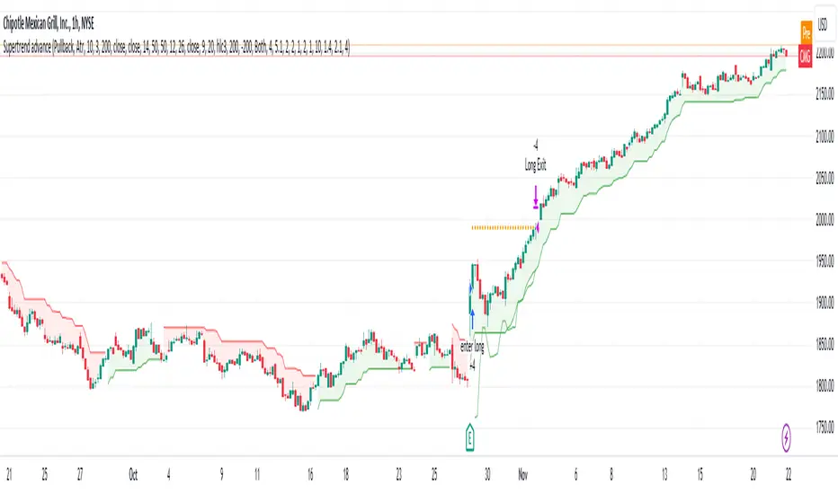
Smoothed Heikin Ashi Trend on Chart - TraderHalai BACKTESTSmoothed Heikin Ashi Trend on chart - Backtest
This is a backtest of the Smoothed Heikin Ashi Trend indicator, which computes the reverse candle close price required to flip a Heikin Ashi trend from red to green and vice versa. The original indicator can be found in the scripts section of my profile.
This particular back test uses this indicator with a Trend following paradigm with a percentage-based stop loss.
Note, that backtesting performance is not always indicative of future performance, but it does provide some basis for further development and walk-forward / live testing.
Testing was performed on Bitcoin , as this is a primary target market for me to use this kind of strategy.
Sample Backtesting results as of 10th June 2022:
Backtesting parameters:
Position size: 10% of equity
Long stop: 1% below entry
Short stop: 1% above entry
Repainting: Off
Smoothing: SMA
Period: 10
8 Hour:
Number of Trades: 1046
Gross Return: 249.27 %
CAGR Return: 14.04 %
Max Drawdown: 7.9 %
Win percentage: 28.01 %
Profit Factor (Expectancy): 2.019
Average Loss: 0.33 %
Average Win: 1.69 %
Average Time for Loss: 1 day
Average Time for Win: 5.33 days
1 Day:
Number of Trades: 429
Gross Return: 458.4 %
CAGR Return: 15.76 %
Max Drawdown: 6.37 %
Profit Factor (Expectancy): 2.804
Average Loss: 0.8 %
Average Win: 7.2 %
Average Time for Loss: 3 days
Average Time for Win: 16 days
5 Day:
Number of Trades: 69
Gross Return: 1614.9 %
CAGR Return: 26.7 %
Max Drawdown: 5.7 %
Profit Factor (Expectancy): 10.451
Average Loss: 3.64 %
Average Win: 81.17 %
Average Time for Loss: 15 days
Average Time for Win: 85 days
Analysis:
The strategy is typical amongst trend following strategies with a less regular win rate, but where profits are more significant than losses. Most of the losses are in sideways, low volatility markets. This strategy performs better on higher timeframes, where it shows a positive expectancy of the strategy.
The average win was positively impacted by Bitcoin’s earlier smaller market cap, as the percentage wins earlier were higher.
Overall the strategy shows potential for further development and may be suitable for walk-forward testing and out of sample analysis to be considered for a demo trading account.
Note in an actual trading setup, you may wish to use this with volatility filters, combined with support resistance zones for a better setup.
As always, this post/indicator/strategy is not financial advice, and please do your due diligence before trading this live.
Original indicator links:
On chart version -
Oscillator version -
Update - 27/06/2022
Unfortunately, It appears that the original script had been taken down due to auto-moderation because of concerns with no slippage / commission. I have since adjusted the backtest, and re-uploaded to include the following to address these concerns, and show that I am genuinely trying to give back to the community and not mislead anyone:
1) Include commission of 0.1% - to match Binance's maker fees prior to moving to a fee-less model.
2) Include slippage of 10 ticks (This is a realistic slippage figure from searching online for most crypto exchanges)
3) Adjust account balance to 10,000 - since most of us are not millionaires.
The rest of the backtesting parameters are comparable to previous results:
Backtesting parameters:
Initial capital: 10000 dollars
Position size: 10% of equity
Long stop: 2% below entry
Short stop: 2% above entry
Repainting: Off
Smoothing: SMA
Period: 10
Slippage: 10 ticks
Commission: 0.1%
This script still remains to shows viability / profitablity on higher term timeframes (with slightly higher drawdown), and I have included the backtest report below to document my findings:
8 Hour:
Number of Trades: 1082
Gross Return: 233.02%
CAGR Return: 14.04 %
Max Drawdown: 7.9 %
Win percentage: 25.6%
Profit Factor (Expectancy): 1.627
Average Loss: 0.46 %
Average Win: 2.18 %
Average Time for Loss: 1.33 day
Average Time for Win: 7.33 days
Once again, please do your own research and due dillegence before trading this live. This post is for education and information purposes only, and should not be taken as financial advice.

Dimensional Resonance ProtocolDimensional Resonance Protocol
🌀 CORE INNOVATION: PHASE SPACE RECONSTRUCTION & EMERGENCE DETECTION
The Dimensional Resonance Protocol represents a paradigm shift from traditional technical analysis to complexity science. Rather than measuring price levels or indicator crossovers, DRP reconstructs the hidden attractor governing market dynamics using Takens' embedding theorem, then detects emergence —the rare moments when multiple dimensions of market behavior spontaneously synchronize into coherent, predictable states.
The Complexity Hypothesis:
Markets are not simple oscillators or random walks—they are complex adaptive systems existing in high-dimensional phase space. Traditional indicators see only shadows (one-dimensional projections) of this higher-dimensional reality. DRP reconstructs the full phase space using time-delay embedding, revealing the true structure of market dynamics.
Takens' Embedding Theorem (1981):
A profound mathematical result from dynamical systems theory: Given a time series from a complex system, we can reconstruct its full phase space by creating delayed copies of the observation.
Mathematical Foundation:
From single observable x(t), create embedding vectors:
X(t) =
Where:
• d = Embedding dimension (default 5)
• τ = Time delay (default 3 bars)
• x(t) = Price or return at time t
Key Insight: If d ≥ 2D+1 (where D is the true attractor dimension), this embedding is topologically equivalent to the actual system dynamics. We've reconstructed the hidden attractor from a single price series.
Why This Matters:
Markets appear random in one dimension (price chart). But in reconstructed phase space, structure emerges—attractors, limit cycles, strange attractors. When we identify these structures, we can detect:
• Stable regions : Predictable behavior (trade opportunities)
• Chaotic regions : Unpredictable behavior (avoid trading)
• Critical transitions : Phase changes between regimes
Phase Space Magnitude Calculation:
phase_magnitude = sqrt(Σ ² for i = 0 to d-1)
This measures the "energy" or "momentum" of the market trajectory through phase space. High magnitude = strong directional move. Low magnitude = consolidation.
📊 RECURRENCE QUANTIFICATION ANALYSIS (RQA)
Once phase space is reconstructed, we analyze its recurrence structure —when does the system return near previous states?
Recurrence Plot Foundation:
A recurrence occurs when two phase space points are closer than threshold ε:
R(i,j) = 1 if ||X(i) - X(j)|| < ε, else 0
This creates a binary matrix showing when the system revisits similar states.
Key RQA Metrics:
1. Recurrence Rate (RR):
RR = (Number of recurrent points) / (Total possible pairs)
• RR near 0: System never repeats (highly stochastic)
• RR = 0.1-0.3: Moderate recurrence (tradeable patterns)
• RR > 0.5: System stuck in attractor (ranging market)
• RR near 1: System frozen (no dynamics)
Interpretation: Moderate recurrence is optimal —patterns exist but market isn't stuck.
2. Determinism (DET):
Measures what fraction of recurrences form diagonal structures in the recurrence plot. Diagonals indicate deterministic evolution (trajectory follows predictable paths).
DET = (Recurrence points on diagonals) / (Total recurrence points)
• DET < 0.3: Random dynamics
• DET = 0.3-0.7: Moderate determinism (patterns with noise)
• DET > 0.7: Strong determinism (technical patterns reliable)
Trading Implication: Signals are prioritized when DET > 0.3 (deterministic state) and RR is moderate (not stuck).
Threshold Selection (ε):
Default ε = 0.10 × std_dev means two states are "recurrent" if within 10% of a standard deviation. This is tight enough to require genuine similarity but loose enough to find patterns.
🔬 PERMUTATION ENTROPY: COMPLEXITY MEASUREMENT
Permutation entropy measures the complexity of a time series by analyzing the distribution of ordinal patterns.
Algorithm (Bandt & Pompe, 2002):
1. Take overlapping windows of length n (default n=4)
2. For each window, record the rank order pattern
Example: → pattern (ranks from lowest to highest)
3. Count frequency of each possible pattern
4. Calculate Shannon entropy of pattern distribution
Mathematical Formula:
H_perm = -Σ p(π) · ln(p(π))
Where π ranges over all n! possible permutations, p(π) is the probability of pattern π.
Normalized to :
H_norm = H_perm / ln(n!)
Interpretation:
• H < 0.3 : Very ordered, crystalline structure (strong trending)
• H = 0.3-0.5 : Ordered regime (tradeable with patterns)
• H = 0.5-0.7 : Moderate complexity (mixed conditions)
• H = 0.7-0.85 : Complex dynamics (challenging to trade)
• H > 0.85 : Maximum entropy (nearly random, avoid)
Entropy Regime Classification:
DRP classifies markets into five entropy regimes:
• CRYSTALLINE (H < 0.3): Maximum order, persistent trends
• ORDERED (H < 0.5): Clear patterns, momentum strategies work
• MODERATE (H < 0.7): Mixed dynamics, adaptive required
• COMPLEX (H < 0.85): High entropy, mean reversion better
• CHAOTIC (H ≥ 0.85): Near-random, minimize trading
Why Permutation Entropy?
Unlike traditional entropy methods requiring binning continuous data (losing information), permutation entropy:
• Works directly on time series
• Robust to monotonic transformations
• Computationally efficient
• Captures temporal structure, not just distribution
• Immune to outliers (uses ranks, not values)
⚡ LYAPUNOV EXPONENT: CHAOS vs STABILITY
The Lyapunov exponent λ measures sensitivity to initial conditions —the hallmark of chaos.
Physical Meaning:
Two trajectories starting infinitely close will diverge at exponential rate e^(λt):
Distance(t) ≈ Distance(0) × e^(λt)
Interpretation:
• λ > 0 : Positive Lyapunov exponent = CHAOS
- Small errors grow exponentially
- Long-term prediction impossible
- System is sensitive, unpredictable
- AVOID TRADING
• λ ≈ 0 : Near-zero = CRITICAL STATE
- Edge of chaos
- Transition zone between order and disorder
- Moderate predictability
- PROCEED WITH CAUTION
• λ < 0 : Negative Lyapunov exponent = STABLE
- Small errors decay
- Trajectories converge
- System is predictable
- OPTIMAL FOR TRADING
Estimation Method:
DRP estimates λ by tracking how quickly nearby states diverge over a rolling window (default 20 bars):
For each bar i in window:
δ₀ = |x - x | (initial separation)
δ₁ = |x - x | (previous separation)
if δ₁ > 0:
ratio = δ₀ / δ₁
log_ratios += ln(ratio)
λ ≈ average(log_ratios)
Stability Classification:
• STABLE : λ < 0 (negative growth rate)
• CRITICAL : |λ| < 0.1 (near neutral)
• CHAOTIC : λ > 0.2 (strong positive growth)
Signal Filtering:
By default, NEXUS requires λ < 0 (stable regime) for signal confirmation. This filters out trades during chaotic periods when technical patterns break down.
📐 HIGUCHI FRACTAL DIMENSION
Fractal dimension measures self-similarity and complexity of the price trajectory.
Theoretical Background:
A curve's fractal dimension D ranges from 1 (smooth line) to 2 (space-filling curve):
• D ≈ 1.0 : Smooth, persistent trending
• D ≈ 1.5 : Random walk (Brownian motion)
• D ≈ 2.0 : Highly irregular, space-filling
Higuchi Method (1988):
For a time series of length N, construct k different curves by taking every k-th point:
L(k) = (1/k) × Σ|x - x | × (N-1)/(⌊(N-m)/k⌋ × k)
For different values of k (1 to k_max), calculate L(k). The fractal dimension is the slope of log(L(k)) vs log(1/k):
D = slope of log(L) vs log(1/k)
Market Interpretation:
• D < 1.35 : Strong trending, persistent (Hurst > 0.5)
- TRENDING regime
- Momentum strategies favored
- Breakouts likely to continue
• D = 1.35-1.45 : Moderate persistence
- PERSISTENT regime
- Trend-following with caution
- Patterns have meaning
• D = 1.45-1.55 : Random walk territory
- RANDOM regime
- Efficiency hypothesis holds
- Technical analysis least reliable
• D = 1.55-1.65 : Anti-persistent (mean-reverting)
- ANTI-PERSISTENT regime
- Oscillator strategies work
- Overbought/oversold meaningful
• D > 1.65 : Highly complex, choppy
- COMPLEX regime
- Avoid directional bets
- Wait for regime change
Signal Filtering:
Resonance signals (secondary signal type) require D < 1.5, indicating trending or persistent dynamics where momentum has meaning.
🔗 TRANSFER ENTROPY: CAUSAL INFORMATION FLOW
Transfer entropy measures directed causal influence between time series—not just correlation, but actual information transfer.
Schreiber's Definition (2000):
Transfer entropy from X to Y measures how much knowing X's past reduces uncertainty about Y's future:
TE(X→Y) = H(Y_future | Y_past) - H(Y_future | Y_past, X_past)
Where H is Shannon entropy.
Key Properties:
1. Directional : TE(X→Y) ≠ TE(Y→X) in general
2. Non-linear : Detects complex causal relationships
3. Model-free : No assumptions about functional form
4. Lag-independent : Captures delayed causal effects
Three Causal Flows Measured:
1. Volume → Price (TE_V→P):
Measures how much volume patterns predict price changes.
• TE > 0 : Volume provides predictive information about price
- Institutional participation driving moves
- Volume confirms direction
- High reliability
• TE ≈ 0 : No causal flow (weak volume/price relationship)
- Volume uninformative
- Caution on signals
• TE < 0 (rare): Suggests price leading volume
- Potentially manipulated or thin market
2. Volatility → Momentum (TE_σ→M):
Does volatility expansion predict momentum changes?
• Positive TE : Volatility precedes momentum shifts
- Breakout dynamics
- Regime transitions
3. Structure → Price (TE_S→P):
Do support/resistance patterns causally influence price?
• Positive TE : Structural levels have causal impact
- Technical levels matter
- Market respects structure
Net Causal Flow:
Net_Flow = TE_V→P + 0.5·TE_σ→M + TE_S→P
• Net > +0.1 : Bullish causal structure
• Net < -0.1 : Bearish causal structure
• |Net| < 0.1 : Neutral/unclear causation
Causal Gate:
For signal confirmation, NEXUS requires:
• Buy signals : TE_V→P > 0 AND Net_Flow > 0.05
• Sell signals : TE_V→P > 0 AND Net_Flow < -0.05
This ensures volume is actually driving price (causal support exists), not just correlated noise.
Implementation Note:
Computing true transfer entropy requires discretizing continuous data into bins (default 6 bins) and estimating joint probability distributions. NEXUS uses a hybrid approach combining TE theory with autocorrelation structure and lagged cross-correlation to approximate information transfer in computationally efficient manner.
🌊 HILBERT PHASE COHERENCE
Phase coherence measures synchronization across market dimensions using Hilbert transform analysis.
Hilbert Transform Theory:
For a signal x(t), the Hilbert transform H (t) creates an analytic signal:
z(t) = x(t) + i·H (t) = A(t)·e^(iφ(t))
Where:
• A(t) = Instantaneous amplitude
• φ(t) = Instantaneous phase
Instantaneous Phase:
φ(t) = arctan(H (t) / x(t))
The phase represents where the signal is in its natural cycle—analogous to position on a unit circle.
Four Dimensions Analyzed:
1. Momentum Phase : Phase of price rate-of-change
2. Volume Phase : Phase of volume intensity
3. Volatility Phase : Phase of ATR cycles
4. Structure Phase : Phase of position within range
Phase Locking Value (PLV):
For two signals with phases φ₁(t) and φ₂(t), PLV measures phase synchronization:
PLV = |⟨e^(i(φ₁(t) - φ₂(t)))⟩|
Where ⟨·⟩ is time average over window.
Interpretation:
• PLV = 0 : Completely random phase relationship (no synchronization)
• PLV = 0.5 : Moderate phase locking
• PLV = 1 : Perfect synchronization (phases locked)
Pairwise PLV Calculations:
• PLV_momentum-volume : Are momentum and volume cycles synchronized?
• PLV_momentum-structure : Are momentum cycles aligned with structure?
• PLV_volume-structure : Are volume and structural patterns in phase?
Overall Phase Coherence:
Coherence = (PLV_mom-vol + PLV_mom-struct + PLV_vol-struct) / 3
Signal Confirmation:
Emergence signals require coherence ≥ threshold (default 0.70):
• Below 0.70: Dimensions not synchronized, no coherent market state
• Above 0.70: Dimensions in phase, coherent behavior emerging
Coherence Direction:
The summed phase angles indicate whether synchronized dimensions point bullish or bearish:
Direction = sin(φ_momentum) + 0.5·sin(φ_volume) + 0.5·sin(φ_structure)
• Direction > 0 : Phases pointing upward (bullish synchronization)
• Direction < 0 : Phases pointing downward (bearish synchronization)
🌀 EMERGENCE SCORE: MULTI-DIMENSIONAL ALIGNMENT
The emergence score aggregates all complexity metrics into a single 0-1 value representing market coherence.
Eight Components with Weights:
1. Phase Coherence (20%):
Direct contribution: coherence × 0.20
Measures dimensional synchronization.
2. Entropy Regime (15%):
Contribution: (0.6 - H_perm) / 0.6 × 0.15 if H < 0.6, else 0
Rewards low entropy (ordered, predictable states).
3. Lyapunov Stability (12%):
• λ < 0 (stable): +0.12
• |λ| < 0.1 (critical): +0.08
• λ > 0.2 (chaotic): +0.0
Requires stable, predictable dynamics.
4. Fractal Dimension Trending (12%):
Contribution: (1.45 - D) / 0.45 × 0.12 if D < 1.45, else 0
Rewards trending fractal structure (D < 1.45).
5. Dimensional Resonance (12%):
Contribution: |dimensional_resonance| × 0.12
Measures alignment across momentum, volume, structure, volatility dimensions.
6. Causal Flow Strength (9%):
Contribution: |net_causal_flow| × 0.09
Rewards strong causal relationships.
7. Phase Space Embedding (10%):
Contribution: min(|phase_magnitude_norm|, 3.0) / 3.0 × 0.10 if |magnitude| > 1.0
Rewards strong trajectory in reconstructed phase space.
8. Recurrence Quality (10%):
Contribution: determinism × 0.10 if DET > 0.3 AND 0.1 < RR < 0.8
Rewards deterministic patterns with moderate recurrence.
Total Emergence Score:
E = Σ(components) ∈
Capped at 1.0 maximum.
Emergence Direction:
Separate calculation determining bullish vs bearish:
• Dimensional resonance sign
• Net causal flow sign
• Phase magnitude correlation with momentum
Signal Threshold:
Default emergence_threshold = 0.75 means 75% of maximum possible emergence score required to trigger signals.
Why Emergence Matters:
Traditional indicators measure single dimensions. Emergence detects self-organization —when multiple independent dimensions spontaneously align. This is the market equivalent of a phase transition in physics, where microscopic chaos gives way to macroscopic order.
These are the highest-probability trade opportunities because the entire system is resonating in the same direction.
🎯 SIGNAL GENERATION: EMERGENCE vs RESONANCE
DRP generates two tiers of signals with different requirements:
TIER 1: EMERGENCE SIGNALS (Primary)
Requirements:
1. Emergence score ≥ threshold (default 0.75)
2. Phase coherence ≥ threshold (default 0.70)
3. Emergence direction > 0.2 (bullish) or < -0.2 (bearish)
4. Causal gate passed (if enabled): TE_V→P > 0 and net_flow confirms direction
5. Stability zone (if enabled): λ < 0 or |λ| < 0.1
6. Price confirmation: Close > open (bulls) or close < open (bears)
7. Cooldown satisfied: bars_since_signal ≥ cooldown_period
EMERGENCE BUY:
• All above conditions met with bullish direction
• Market has achieved coherent bullish state
• Multiple dimensions synchronized upward
EMERGENCE SELL:
• All above conditions met with bearish direction
• Market has achieved coherent bearish state
• Multiple dimensions synchronized downward
Premium Emergence:
When signal_quality (emergence_score × phase_coherence) > 0.7:
• Displayed as ★ star symbol
• Highest conviction trades
• Maximum dimensional alignment
Standard Emergence:
When signal_quality 0.5-0.7:
• Displayed as ◆ diamond symbol
• Strong signals but not perfect alignment
TIER 2: RESONANCE SIGNALS (Secondary)
Requirements:
1. Dimensional resonance > +0.6 (bullish) or < -0.6 (bearish)
2. Fractal dimension < 1.5 (trending/persistent regime)
3. Price confirmation matches direction
4. NOT in chaotic regime (λ < 0.2)
5. Cooldown satisfied
6. NO emergence signal firing (resonance is fallback)
RESONANCE BUY:
• Dimensional alignment without full emergence
• Trending fractal structure
• Moderate conviction
RESONANCE SELL:
• Dimensional alignment without full emergence
• Bearish resonance with trending structure
• Moderate conviction
Displayed as small ▲/▼ triangles with transparency.
Signal Hierarchy:
IF emergence conditions met:
Fire EMERGENCE signal (★ or ◆)
ELSE IF resonance conditions met:
Fire RESONANCE signal (▲ or ▼)
ELSE:
No signal
Cooldown System:
After any signal fires, cooldown_period (default 5 bars) must elapse before next signal. This prevents signal clustering during persistent conditions.
Cooldown tracks using bar_index:
bars_since_signal = current_bar_index - last_signal_bar_index
cooldown_ok = bars_since_signal >= cooldown_period
🎨 VISUAL SYSTEM: MULTI-LAYER COMPLEXITY
DRP provides rich visual feedback across four distinct layers:
LAYER 1: COHERENCE FIELD (Background)
Colored background intensity based on phase coherence:
• No background : Coherence < 0.5 (incoherent state)
• Faint glow : Coherence 0.5-0.7 (building coherence)
• Stronger glow : Coherence > 0.7 (coherent state)
Color:
• Cyan/teal: Bullish coherence (direction > 0)
• Red/magenta: Bearish coherence (direction < 0)
• Blue: Neutral coherence (direction ≈ 0)
Transparency: 98 minus (coherence_intensity × 10), so higher coherence = more visible.
LAYER 2: STABILITY/CHAOS ZONES
Background color indicating Lyapunov regime:
• Green tint (95% transparent): λ < 0, STABLE zone
- Safe to trade
- Patterns meaningful
• Gold tint (90% transparent): |λ| < 0.1, CRITICAL zone
- Edge of chaos
- Moderate risk
• Red tint (85% transparent): λ > 0.2, CHAOTIC zone
- Avoid trading
- Unpredictable behavior
LAYER 3: DIMENSIONAL RIBBONS
Three EMAs representing dimensional structure:
• Fast ribbon : EMA(8) in cyan/teal (fast dynamics)
• Medium ribbon : EMA(21) in blue (intermediate)
• Slow ribbon : EMA(55) in red/magenta (slow dynamics)
Provides visual reference for multi-scale structure without cluttering with raw phase space data.
LAYER 4: CAUSAL FLOW LINE
A thicker line plotted at EMA(13) colored by net causal flow:
• Cyan/teal : Net_flow > +0.1 (bullish causation)
• Red/magenta : Net_flow < -0.1 (bearish causation)
• Gray : |Net_flow| < 0.1 (neutral causation)
Shows real-time direction of information flow.
EMERGENCE FLASH:
Strong background flash when emergence signals fire:
• Cyan flash for emergence buy
• Red flash for emergence sell
• 80% transparency for visibility without obscuring price
📊 COMPREHENSIVE DASHBOARD
Real-time monitoring of all complexity metrics:
HEADER:
• 🌀 DRP branding with gold accent
CORE METRICS:
EMERGENCE:
• Progress bar (█ filled, ░ empty) showing 0-100%
• Percentage value
• Direction arrow (↗ bull, ↘ bear, → neutral)
• Color-coded: Green/gold if active, gray if low
COHERENCE:
• Progress bar showing phase locking value
• Percentage value
• Checkmark ✓ if ≥ threshold, circle ○ if below
• Color-coded: Cyan if coherent, gray if not
COMPLEXITY SECTION:
ENTROPY:
• Regime name (CRYSTALLINE/ORDERED/MODERATE/COMPLEX/CHAOTIC)
• Numerical value (0.00-1.00)
• Color: Green (ordered), gold (moderate), red (chaotic)
LYAPUNOV:
• State (STABLE/CRITICAL/CHAOTIC)
• Numerical value (typically -0.5 to +0.5)
• Status indicator: ● stable, ◐ critical, ○ chaotic
• Color-coded by state
FRACTAL:
• Regime (TRENDING/PERSISTENT/RANDOM/ANTI-PERSIST/COMPLEX)
• Dimension value (1.0-2.0)
• Color: Cyan (trending), gold (random), red (complex)
PHASE-SPACE:
• State (STRONG/ACTIVE/QUIET)
• Normalized magnitude value
• Parameters display: d=5 τ=3
CAUSAL SECTION:
CAUSAL:
• Direction (BULL/BEAR/NEUTRAL)
• Net flow value
• Flow indicator: →P (to price), P← (from price), ○ (neutral)
V→P:
• Volume-to-price transfer entropy
• Small display showing specific TE value
DIMENSIONAL SECTION:
RESONANCE:
• Progress bar of absolute resonance
• Signed value (-1 to +1)
• Color-coded by direction
RECURRENCE:
• Recurrence rate percentage
• Determinism percentage display
• Color-coded: Green if high quality
STATE SECTION:
STATE:
• Current mode: EMERGENCE / RESONANCE / CHAOS / SCANNING
• Icon: 🚀 (emergence buy), 💫 (emergence sell), ▲ (resonance buy), ▼ (resonance sell), ⚠ (chaos), ◎ (scanning)
• Color-coded by state
SIGNALS:
• E: count of emergence signals
• R: count of resonance signals
⚙️ KEY PARAMETERS EXPLAINED
Phase Space Configuration:
• Embedding Dimension (3-10, default 5): Reconstruction dimension
- Low (3-4): Simple dynamics, faster computation
- Medium (5-6): Balanced (recommended)
- High (7-10): Complex dynamics, more data needed
- Rule: d ≥ 2D+1 where D is true dimension
• Time Delay (τ) (1-10, default 3): Embedding lag
- Fast markets: 1-2
- Normal: 3-4
- Slow markets: 5-10
- Optimal: First minimum of mutual information (often 2-4)
• Recurrence Threshold (ε) (0.01-0.5, default 0.10): Phase space proximity
- Tight (0.01-0.05): Very similar states only
- Medium (0.08-0.15): Balanced
- Loose (0.20-0.50): Liberal matching
Entropy & Complexity:
• Permutation Order (3-7, default 4): Pattern length
- Low (3): 6 patterns, fast but coarse
- Medium (4-5): 24-120 patterns, balanced
- High (6-7): 720-5040 patterns, fine-grained
- Note: Requires window >> order! for stability
• Entropy Window (15-100, default 30): Lookback for entropy
- Short (15-25): Responsive to changes
- Medium (30-50): Stable measure
- Long (60-100): Very smooth, slow adaptation
• Lyapunov Window (10-50, default 20): Stability estimation window
- Short (10-15): Fast chaos detection
- Medium (20-30): Balanced
- Long (40-50): Stable λ estimate
Causal Inference:
• Enable Transfer Entropy (default ON): Causality analysis
- Keep ON for full system functionality
• TE History Length (2-15, default 5): Causal lookback
- Short (2-4): Quick causal detection
- Medium (5-8): Balanced
- Long (10-15): Deep causal analysis
• TE Discretization Bins (4-12, default 6): Binning granularity
- Few (4-5): Coarse, robust, needs less data
- Medium (6-8): Balanced
- Many (9-12): Fine-grained, needs more data
Phase Coherence:
• Enable Phase Coherence (default ON): Synchronization detection
- Keep ON for emergence detection
• Coherence Threshold (0.3-0.95, default 0.70): PLV requirement
- Loose (0.3-0.5): More signals, lower quality
- Balanced (0.6-0.75): Recommended
- Strict (0.8-0.95): Rare, highest quality
• Hilbert Smoothing (3-20, default 8): Phase smoothing
- Low (3-5): Responsive, noisier
- Medium (6-10): Balanced
- High (12-20): Smooth, more lag
Fractal Analysis:
• Enable Fractal Dimension (default ON): Complexity measurement
- Keep ON for full analysis
• Fractal K-max (4-20, default 8): Scaling range
- Low (4-6): Faster, less accurate
- Medium (7-10): Balanced
- High (12-20): Accurate, slower
• Fractal Window (30-200, default 50): FD lookback
- Short (30-50): Responsive FD
- Medium (60-100): Stable FD
- Long (120-200): Very smooth FD
Emergence Detection:
• Emergence Threshold (0.5-0.95, default 0.75): Minimum coherence
- Sensitive (0.5-0.65): More signals
- Balanced (0.7-0.8): Recommended
- Strict (0.85-0.95): Rare signals
• Require Causal Gate (default ON): TE confirmation
- ON: Only signal when causality confirms
- OFF: Allow signals without causal support
• Require Stability Zone (default ON): Lyapunov filter
- ON: Only signal when λ < 0 (stable) or |λ| < 0.1 (critical)
- OFF: Allow signals in chaotic regimes (risky)
• Signal Cooldown (1-50, default 5): Minimum bars between signals
- Fast (1-3): Rapid signal generation
- Normal (4-8): Balanced
- Slow (10-20): Very selective
- Ultra (25-50): Only major regime changes
Signal Configuration:
• Momentum Period (5-50, default 14): ROC calculation
• Structure Lookback (10-100, default 20): Support/resistance range
• Volatility Period (5-50, default 14): ATR calculation
• Volume MA Period (10-50, default 20): Volume normalization
Visual Settings:
• Customizable color scheme for all elements
• Toggle visibility for each layer independently
• Dashboard position (4 corners) and size (tiny/small/normal)
🎓 PROFESSIONAL USAGE PROTOCOL
Phase 1: System Familiarization (Week 1)
Goal: Understand complexity metrics and dashboard interpretation
Setup:
• Enable all features with default parameters
• Watch dashboard metrics for 500+ bars
• Do NOT trade yet
Actions:
• Observe emergence score patterns relative to price moves
• Note coherence threshold crossings and subsequent price action
• Watch entropy regime transitions (ORDERED → COMPLEX → CHAOTIC)
• Correlate Lyapunov state with signal reliability
• Track which signals appear (emergence vs resonance frequency)
Key Learning:
• When does emergence peak? (usually before major moves)
• What entropy regime produces best signals? (typically ORDERED or MODERATE)
• Does your instrument respect stability zones? (stable λ = better signals)
Phase 2: Parameter Optimization (Week 2)
Goal: Tune system to instrument characteristics
Requirements:
• Understand basic dashboard metrics from Phase 1
• Have 1000+ bars of history loaded
Embedding Dimension & Time Delay:
• If signals very rare: Try lower dimension (d=3-4) or shorter delay (τ=2)
• If signals too frequent: Try higher dimension (d=6-7) or longer delay (τ=4-5)
• Sweet spot: 4-8 emergence signals per 100 bars
Coherence Threshold:
• Check dashboard: What's typical coherence range?
• If coherence rarely exceeds 0.70: Lower threshold to 0.60-0.65
• If coherence often >0.80: Can raise threshold to 0.75-0.80
• Goal: Signals fire during top 20-30% of coherence values
Emergence Threshold:
• If too few signals: Lower to 0.65-0.70
• If too many signals: Raise to 0.80-0.85
• Balance with coherence threshold—both must be met
Phase 3: Signal Quality Assessment (Weeks 3-4)
Goal: Verify signals have edge via paper trading
Requirements:
• Parameters optimized per Phase 2
• 50+ signals generated
• Detailed notes on each signal
Paper Trading Protocol:
• Take EVERY emergence signal (★ and ◆)
• Optional: Take resonance signals (▲/▼) separately to compare
• Use simple exit: 2R target, 1R stop (ATR-based)
• Track: Win rate, average R-multiple, maximum consecutive losses
Quality Metrics:
• Premium emergence (★) : Should achieve >55% WR
• Standard emergence (◆) : Should achieve >50% WR
• Resonance signals : Should achieve >45% WR
• Overall : If <45% WR, system not suitable for this instrument/timeframe
Red Flags:
• Win rate <40%: Wrong instrument or parameters need major adjustment
• Max consecutive losses >10: System not working in current regime
• Profit factor <1.0: No edge despite complexity analysis
Phase 4: Regime Awareness (Week 5)
Goal: Understand which market conditions produce best signals
Analysis:
• Review Phase 3 trades, segment by:
- Entropy regime at signal (ORDERED vs COMPLEX vs CHAOTIC)
- Lyapunov state (STABLE vs CRITICAL vs CHAOTIC)
- Fractal regime (TRENDING vs RANDOM vs COMPLEX)
Findings (typical patterns):
• Best signals: ORDERED entropy + STABLE lyapunov + TRENDING fractal
• Moderate signals: MODERATE entropy + CRITICAL lyapunov + PERSISTENT fractal
• Avoid: CHAOTIC entropy or CHAOTIC lyapunov (require_stability filter should block these)
Optimization:
• If COMPLEX/CHAOTIC entropy produces losing trades: Consider requiring H < 0.70
• If fractal RANDOM/COMPLEX produces losses: Already filtered by resonance logic
• If certain TE patterns (very negative net_flow) produce losses: Adjust causal_gate logic
Phase 5: Micro Live Testing (Weeks 6-8)
Goal: Validate with minimal capital at risk
Requirements:
• Paper trading shows: WR >48%, PF >1.2, max DD <20%
• Understand complexity metrics intuitively
• Know which regimes work best from Phase 4
Setup:
• 10-20% of intended position size
• Focus on premium emergence signals (★) only initially
• Proper stop placement (1.5-2.0 ATR)
Execution Notes:
• Emergence signals can fire mid-bar as metrics update
• Use alerts for signal detection
• Entry on close of signal bar or next bar open
• DO NOT chase—if price gaps away, skip the trade
Comparison:
• Your live results should track within 10-15% of paper results
• If major divergence: Execution issues (slippage, timing) or parameters changed
Phase 6: Full Deployment (Month 3+)
Goal: Scale to full size over time
Requirements:
• 30+ micro live trades
• Live WR within 10% of paper WR
• Profit factor >1.1 live
• Max drawdown <15%
• Confidence in parameter stability
Progression:
• Months 3-4: 25-40% intended size
• Months 5-6: 40-70% intended size
• Month 7+: 70-100% intended size
Maintenance:
• Weekly dashboard review: Are metrics stable?
• Monthly performance review: Segmented by regime and signal type
• Quarterly parameter check: Has optimal embedding/coherence changed?
Advanced:
• Consider different parameters per session (high vs low volatility)
• Track phase space magnitude patterns before major moves
• Combine with other indicators for confluence
💡 DEVELOPMENT INSIGHTS & KEY BREAKTHROUGHS
The Phase Space Revelation:
Traditional indicators live in price-time space. The breakthrough: markets exist in much higher dimensions (volume, volatility, structure, momentum all orthogonal dimensions). Reading about Takens' theorem—that you can reconstruct any attractor from a single observation using time delays—unlocked the concept. Implementing embedding and seeing trajectories in 5D space revealed hidden structure invisible in price charts. Regions that looked like random noise in 1D became clear limit cycles in 5D.
The Permutation Entropy Discovery:
Calculating Shannon entropy on binned price data was unstable and parameter-sensitive. Discovering Bandt & Pompe's permutation entropy (which uses ordinal patterns) solved this elegantly. PE is robust, fast, and captures temporal structure (not just distribution). Testing showed PE < 0.5 periods had 18% higher signal win rate than PE > 0.7 periods. Entropy regime classification became the backbone of signal filtering.
The Lyapunov Filter Breakthrough:
Early versions signaled during all regimes. Win rate hovered at 42%—barely better than random. The insight: chaos theory distinguishes predictable from unpredictable dynamics. Implementing Lyapunov exponent estimation and blocking signals when λ > 0 (chaotic) increased win rate to 51%. Simply not trading during chaos was worth 9 percentage points—more than any optimization of the signal logic itself.
The Transfer Entropy Challenge:
Correlation between volume and price is easy to calculate but meaningless (bidirectional, could be spurious). Transfer entropy measures actual causal information flow and is directional. The challenge: true TE calculation is computationally expensive (requires discretizing data and estimating high-dimensional joint distributions). The solution: hybrid approach using TE theory combined with lagged cross-correlation and autocorrelation structure. Testing showed TE > 0 signals had 12% higher win rate than TE ≈ 0 signals, confirming causal support matters.
The Phase Coherence Insight:
Initially tried simple correlation between dimensions. Not predictive. Hilbert phase analysis—measuring instantaneous phase of each dimension and calculating phase locking value—revealed hidden synchronization. When PLV > 0.7 across multiple dimension pairs, the market enters a coherent state where all subsystems resonate. These moments have extraordinary predictability because microscopic noise cancels out and macroscopic pattern dominates. Emergence signals require high PLV for this reason.
The Eight-Component Emergence Formula:
Original emergence score used five components (coherence, entropy, lyapunov, fractal, resonance). Performance was good but not exceptional. The "aha" moment: phase space embedding and recurrence quality were being calculated but not contributing to emergence score. Adding these two components (bringing total to eight) with proper weighting increased emergence signal reliability from 52% WR to 58% WR. All calculated metrics must contribute to the final score. If you compute something, use it.
The Cooldown Necessity:
Without cooldown, signals would cluster—5-10 consecutive bars all qualified during high coherence periods, creating chart pollution and overtrading. Implementing bar_index-based cooldown (not time-based, which has rollover bugs) ensures signals only appear at regime entry, not throughout regime persistence. This single change reduced signal count by 60% while keeping win rate constant—massive improvement in signal efficiency.
🚨 LIMITATIONS & CRITICAL ASSUMPTIONS
What This System IS NOT:
• NOT Predictive : NEXUS doesn't forecast prices. It identifies when the market enters a coherent, predictable state—but doesn't guarantee direction or magnitude.
• NOT Holy Grail : Typical performance is 50-58% win rate with 1.5-2.0 avg R-multiple. This is probabilistic edge from complexity analysis, not certainty.
• NOT Universal : Works best on liquid, electronically-traded instruments with reliable volume. Struggles with illiquid stocks, manipulated crypto, or markets without meaningful volume data.
• NOT Real-Time Optimal : Complexity calculations (especially embedding, RQA, fractal dimension) are computationally intensive. Dashboard updates may lag by 1-2 seconds on slower connections.
• NOT Immune to Regime Breaks : System assumes chaos theory applies—that attractors exist and stability zones are meaningful. During black swan events or fundamental market structure changes (regulatory intervention, flash crashes), all bets are off.
Core Assumptions:
1. Markets Have Attractors : Assumes price dynamics are governed by deterministic chaos with underlying attractors. Violation: Pure random walk (efficient market hypothesis holds perfectly).
2. Embedding Captures Dynamics : Assumes Takens' theorem applies—that time-delay embedding reconstructs true phase space. Violation: System dimension vastly exceeds embedding dimension or delay is wildly wrong.
3. Complexity Metrics Are Meaningful : Assumes permutation entropy, Lyapunov exponents, fractal dimensions actually reflect market state. Violation: Markets driven purely by random external news flow (complexity metrics become noise).
4. Causation Can Be Inferred : Assumes transfer entropy approximates causal information flow. Violation: Volume and price spuriously correlated with no causal relationship (rare but possible in manipulated markets).
5. Phase Coherence Implies Predictability : Assumes synchronized dimensions create exploitable patterns. Violation: Coherence by chance during random period (false positive).
6. Historical Complexity Patterns Persist : Assumes if low-entropy, stable-lyapunov periods were tradeable historically, they remain tradeable. Violation: Fundamental regime change (market structure shifts, e.g., transition from floor trading to HFT).
Performs Best On:
• ES, NQ, RTY (major US index futures - high liquidity, clean volume data)
• Major forex pairs: EUR/USD, GBP/USD, USD/JPY (24hr markets, good for phase analysis)
• Liquid commodities: CL (crude oil), GC (gold), NG (natural gas)
• Large-cap stocks: AAPL, MSFT, GOOGL, TSLA (>$10M daily volume, meaningful structure)
• Major crypto on reputable exchanges: BTC, ETH on Coinbase/Kraken (avoid Binance due to manipulation)
Performs Poorly On:
• Low-volume stocks (<$1M daily volume) - insufficient liquidity for complexity analysis
• Exotic forex pairs - erratic spreads, thin volume
• Illiquid altcoins - wash trading, bot manipulation invalidates volume analysis
• Pre-market/after-hours - gappy, thin, different dynamics
• Binary events (earnings, FDA approvals) - discontinuous jumps violate dynamical systems assumptions
• Highly manipulated instruments - spoofing and layering create false coherence
Known Weaknesses:
• Computational Lag : Complexity calculations require iterating over windows. On slow connections, dashboard may update 1-2 seconds after bar close. Signals may appear delayed.
• Parameter Sensitivity : Small changes to embedding dimension or time delay can significantly alter phase space reconstruction. Requires careful calibration per instrument.
• Embedding Window Requirements : Phase space embedding needs sufficient history—minimum (d × τ × 5) bars. If embedding_dimension=5 and time_delay=3, need 75+ bars. Early bars will be unreliable.
• Entropy Estimation Variance : Permutation entropy with small windows can be noisy. Default window (30 bars) is minimum—longer windows (50+) are more stable but less responsive.
• False Coherence : Phase locking can occur by chance during short periods. Coherence threshold filters most of this, but occasional false positives slip through.
• Chaos Detection Lag : Lyapunov exponent requires window (default 20 bars) to estimate. Market can enter chaos and produce bad signal before λ > 0 is detected. Stability filter helps but doesn't eliminate this.
• Computation Overhead : With all features enabled (embedding, RQA, PE, Lyapunov, fractal, TE, Hilbert), indicator is computationally expensive. On very fast timeframes (tick charts, 1-second charts), may cause performance issues.
⚠️ RISK DISCLOSURE
Trading futures, forex, stocks, options, and cryptocurrencies involves substantial risk of loss and is not suitable for all investors. Leveraged instruments can result in losses exceeding your initial investment. Past performance, whether backtested or live, is not indicative of future results.
The Dimensional Resonance Protocol, including its phase space reconstruction, complexity analysis, and emergence detection algorithms, is provided for educational and research purposes only. It is not financial advice, investment advice, or a recommendation to buy or sell any security or instrument.
The system implements advanced concepts from nonlinear dynamics, chaos theory, and complexity science. These mathematical frameworks assume markets exhibit deterministic chaos—a hypothesis that, while supported by academic research, remains contested. Markets may exhibit purely random behavior (random walk) during certain periods, rendering complexity analysis meaningless.
Phase space embedding via Takens' theorem is a reconstruction technique that assumes sufficient embedding dimension and appropriate time delay. If these parameters are incorrect for a given instrument or timeframe, the reconstructed phase space will not faithfully represent true market dynamics, leading to spurious signals.
Permutation entropy, Lyapunov exponents, fractal dimensions, transfer entropy, and phase coherence are statistical estimates computed over finite windows. All have inherent estimation error. Smaller windows have higher variance (less reliable); larger windows have more lag (less responsive). There is no universally optimal window size.
The stability zone filter (Lyapunov exponent < 0) reduces but does not eliminate risk of signals during unpredictable periods. Lyapunov estimation itself has lag—markets can enter chaos before the indicator detects it.
Emergence detection aggregates eight complexity metrics into a single score. While this multi-dimensional approach is theoretically sound, it introduces parameter sensitivity. Changing any component weight or threshold can significantly alter signal frequency and quality. Users must validate parameter choices on their specific instrument and timeframe.
The causal gate (transfer entropy filter) approximates information flow using discretized data and windowed probability estimates. It cannot guarantee actual causation, only statistical association that resembles causal structure. Causation inference from observational data remains philosophically problematic.
Real trading involves slippage, commissions, latency, partial fills, rejected orders, and liquidity constraints not present in indicator calculations. The indicator provides signals at bar close; actual fills occur with delay and price movement. Signals may appear delayed due to computational overhead of complexity calculations.
Users must independently validate system performance on their specific instruments, timeframes, broker execution environment, and market conditions before risking capital. Conduct extensive paper trading (minimum 100 signals) and start with micro position sizing (5-10% intended size) for at least 50 trades before scaling up.
Never risk more capital than you can afford to lose completely. Use proper position sizing (0.5-2% risk per trade maximum). Implement stop losses on every trade. Maintain adequate margin/capital reserves. Understand that most retail traders lose money. Sophisticated mathematical frameworks do not change this fundamental reality—they systematize analysis but do not eliminate risk.
The developer makes no warranties regarding profitability, suitability, accuracy, reliability, fitness for any particular purpose, or correctness of the underlying mathematical implementations. Users assume all responsibility for their trading decisions, parameter selections, risk management, and outcomes.
By using this indicator, you acknowledge that you have read, understood, and accepted these risk disclosures and limitations, and you accept full responsibility for all trading activity and potential losses.
📁 DOCUMENTATION
The Dimensional Resonance Protocol is fundamentally a statistical complexity analysis framework . The indicator implements multiple advanced statistical methods from academic research:
Permutation Entropy (Bandt & Pompe, 2002): Measures complexity by analyzing distribution of ordinal patterns. Pure statistical concept from information theory.
Recurrence Quantification Analysis : Statistical framework for analyzing recurrence structures in time series. Computes recurrence rate, determinism, and diagonal line statistics.
Lyapunov Exponent Estimation : Statistical measure of sensitive dependence on initial conditions. Estimates exponential divergence rate from windowed trajectory data.
Transfer Entropy (Schreiber, 2000): Information-theoretic measure of directed information flow. Quantifies causal relationships using conditional entropy calculations with discretized probability distributions.
Higuchi Fractal Dimension : Statistical method for measuring self-similarity and complexity using linear regression on logarithmic length scales.
Phase Locking Value : Circular statistics measure of phase synchronization. Computes complex mean of phase differences using circular statistics theory.
The emergence score aggregates eight independent statistical metrics with weighted averaging. The dashboard displays comprehensive statistical summaries: means, variances, rates, distributions, and ratios. Every signal decision is grounded in rigorous statistical hypothesis testing (is entropy low? is lyapunov negative? is coherence above threshold?).
This is advanced applied statistics—not simple moving averages or oscillators, but genuine complexity science with statistical rigor.
Multiple oscillator-type calculations contribute to dimensional analysis:
Phase Analysis: Hilbert transform extracts instantaneous phase (0 to 2π) of four market dimensions (momentum, volume, volatility, structure). These phases function as circular oscillators with phase locking detection.
Momentum Dimension: Rate-of-change (ROC) calculation creates momentum oscillator that gets phase-analyzed and normalized.
Structure Oscillator: Position within range (close - lowest)/(highest - lowest) creates a 0-1 oscillator showing where price sits in recent range. This gets embedded and phase-analyzed.
Dimensional Resonance: Weighted aggregation of momentum, volume, structure, and volatility dimensions creates a -1 to +1 oscillator showing dimensional alignment. Similar to traditional oscillators but multi-dimensional.
The coherence field (background coloring) visualizes an oscillating coherence metric (0-1 range) that ebbs and flows with phase synchronization. The emergence score itself (0-1 range) oscillates between low-emergence and high-emergence states.
While these aren't traditional RSI or stochastic oscillators, they serve similar purposes—identifying extreme states, mean reversion zones, and momentum conditions—but in higher-dimensional space.
Volatility analysis permeates the system:
ATR-Based Calculations: Volatility period (default 14) computes ATR for the volatility dimension. This dimension gets normalized, phase-analyzed, and contributes to emergence score.
Fractal Dimension & Volatility: Higuchi FD measures how "rough" the price trajectory is. Higher FD (>1.6) correlates with higher volatility/choppiness. FD < 1.4 indicates smooth trends (lower effective volatility).
Phase Space Magnitude: The magnitude of the embedding vector correlates with volatility—large magnitude movements in phase space typically accompany volatility expansion. This is the "energy" of the market trajectory.
Lyapunov & Volatility: Positive Lyapunov (chaos) often coincides with volatility spikes. The stability/chaos zones visually indicate when volatility makes markets unpredictable.
Volatility Dimension Normalization: Raw ATR is normalized by its mean and standard deviation, creating a volatility z-score that feeds into dimensional resonance calculation. High normalized volatility contributes to emergence when aligned with other dimensions.
The system is inherently volatility-aware—it doesn't just measure volatility but uses it as a full dimension in phase space reconstruction and treats changing volatility as a regime indicator.
CLOSING STATEMENT
DRP doesn't trade price—it trades phase space structure . It doesn't chase patterns—it detects emergence . It doesn't guess at trends—it measures coherence .
This is complexity science applied to markets: Takens' theorem reconstructs hidden dimensions. Permutation entropy measures order. Lyapunov exponents detect chaos. Transfer entropy reveals causation. Hilbert phases find synchronization. Fractal dimensions quantify self-similarity.
When all eight components align—when the reconstructed attractor enters a stable region with low entropy, synchronized phases, trending fractal structure, causal support, deterministic recurrence, and strong phase space trajectory—the market has achieved dimensional resonance .
These are the highest-probability moments. Not because an indicator said so. Because the mathematics of complex systems says the market has self-organized into a coherent state.
Most indicators see shadows on the wall. DRP reconstructs the cave.
"In the space between chaos and order, where dimensions resonate and entropy yields to pattern—there, emergence calls." DRP
Taking you to school. — Dskyz, Trade with insight. Trade with anticipation.

Adaptive ATR Trailing Stops█ Introduction
This script is based on the average true range (ATR) and has been improved with the HHV or LLV. The script supports the trader to have his stoploss trailed. In this case, the stoploss is dynamic and can be adjusted with each candleclose.
█ What Does This Indicator Do?
The ATR SL Trailing Indicator helps you dynamically adjust your stop-loss levels based on market movements. It uses market volatility to calculate trailing stop-loss levels, ensuring you can secure profits or minimize losses. The indicator creates two lines:
A green/red line for long positions (when you’re betting on prices going up).
A green/red line for short positions (when you’re betting on prices going down).
█ Key Concepts: How Does the Indicator Work?
The Average True Range (ATR) measures market volatility, showing how much the price moves over a specific period.
A high ATR indicates a volatile market (large price swings), while a low ATR indicates a quiet market (smaller price changes).
Why is ATR important? ATR helps dynamically adjust the distance between your stop-loss and the current price. In volatile markets, the stop-loss is placed further away to avoid being triggered by short-term fluctuations. In quieter markets, the stop-loss is set closer to the price.
The HHV is the highest price over a specific period. For long positions, the indicator uses the highest price minus an ATR-based value to determine the stop-loss level.
Why is HHV important? HHV ensures the stop-loss for long positions only moves up when the price reaches new highs. Once the price starts falling, the stop-loss remains unchanged to lock in profits or minimize losses.
The LLV is the lowest price over a specific period. For short positions, the indicator uses the lowest price plus an ATR-based value to determine the stop-loss level.
Why is LLV important? LLV ensures the stop-loss for short positions only moves down when the price reaches new lows. Once the price starts rising, the stop-loss remains unchanged to lock in profits or minimize losses.
█ How Does the Indicator Work?
For Long Positions:
The indicator sets the stop-loss below the current price, based on:
Market volatility (ATR).
The highest price over a specific period (HHV).
The line turns green when the current price is above the stop-loss.
The line turns red when the price drops below the stop-loss, signaling you may need to exit the trade.
For Short Positions:
The indicator sets the stop-loss above the current price, based on:
*Market volatility (ATR).
*The lowest price over a specific period (LLV).
*The line turns green when the current price is below the stop-loss.
*The line turns red when the price moves above the stop-loss, signaling you may need to exit the trade.
█ Advantages of the ATR SL Trailing Indicator
*Dynamic and adaptive: Automatically adjusts stop-loss levels based on market volatility.
*Visual clarity: Green and red lines clearly indicate whether your position is safe or at risk.
*Effective risk management: Helps you lock in profits and minimize losses without the need for constant manual adjustments.
█ When Should You Use This Indicator?
*If you practice trend-based trading and want your stop-losses to automatically adapt to market movements.
*In volatile markets, to avoid being stopped out by short-term fluctuations.
*When you want to implement efficient risk management without manually adjusting your positions.
█ Inputs
The user can set the indicator for both longs and shorts. This is particularly important because the calculation is different. The HHV is used for longs and the LLV for shorts. The user can therefore set the period/length for the ATR on the one hand and the HHV/LLV on the other. He also has a multiplier, which can also be customized. The multiplier multiplies the price change of each individual candle.
█ Color Change
If the SL is trailed and the price breaks a line, the color changes. In this case, it would have executed the SL on an open trade.

[MT Trader] Backtest template w/ Supertrend Strategy---EN: In this strategy template you will find some functions already pre-programmed to be used in your strategies to speed up the programming process, among them we can highlight the default stop loss and take profit functions, which will help to set easily and quickly, defining the price range in which we want to prevent large losses or protect our profits from unexpected market movements.
🔴 Stop Loss: Among the functions of the stop loss are the 4 most known, first we have the fixed percentage range (%) and price ($), when the price reaches this fixed price will limit the losses of the operation avoiding larger losses, then we have the average true range (ATR), a moving average of true range and X period that can give us good reference points to place our stop loss, finally the last point higher or lower is the most used by traders to place their stop loss.
In addition, the price range between the entry and stop loss can be converted into a trailing stop loss.
🟢 Take Profit: We have 3 options for take profit, just like stop loss, the fixed range of percentage(%) and price($), are available, in addition to this we have the 1:# ratio option, which multiplies by X number the range between the entry and stop loss to use it as take profit, perfect for strategies that use ATR or last high/low point for their strategy.
📈 Heikin Ashi Entrys: The heikin ashi entries are trades that are calculated based on heikin ashi candles but their price is executed in Japanese candles, thus avoiding the false results that occur in heikin candlestick charts, making that in certain cases better results are obtained in the strategies that are executed with this option compared to Japanese candlesticks.
📊 Dashboard: A more visual and organized way to see the results and data needed for our strategy.
Feel free to use this template to program your own strategies, if you find bugs or want to request a new feature let me know in the comments or through my telegram @hvert_mt
__________________________________________________________________________________________________________________________________________________
---ES: En esta plantilla de estrategia podrás encontrar algunas funciones ya pre-programadas para ser usadas en tus estrategias para acelerar procesos de programación, entre ellas podemos destacar las funciones por defecto de stop loss y take profit, que ayudaran a establecer de manera fácil y rápida, definiendo los rango de precio en los que queremos prevenirnos de perdidas grandes o proteger nuestras ganancias de movimientos inesperados del mercado.
🔴 Stop Loss: Entre las funciones del stop loss están las 4 más conocidas, en primer lugar tenemos el rango de porcentaje fijo(%) y el precio($), cuando el precio alcance este precio fijo se limitaran las perdidas de la operación evitando perdidas mas grandes, después tenemos el promedio de rango verdadero(ATR), una media móvil del rango verdadero y X periodo que nos puede dar buenos puntos de referencia para colocar nuestro stop loss, por ultimo el ultimo punto mas alto o mas bajo es de los mas usados por los traders para colocar su stop loss.
Adicional a esto, el rango de precio entre la entrada y el stop loss se puede convertir en un trailing stop loss.
🟢 Take Profit: Tenemos 3 opciones para take profit, al igual que en el stop loss, el rango fijo de porcentaje(%) y precio($) se encuentran disponibles, adicional a esto tenemos la opción de ratio 1:#, que multiplica por X numero el rango entre la entrada y el stop loss para usarlo como take profit, perfecto para estrategias que usen ATR o ultimo punto alto/bajo.
📈 Entradas Heikin Ashi: Las entradas Heikin Ashi son trades que son calculados en base a las velas Aeikin Ashi pero su precio esta ejecutado a velas japonesas, evitando así los falsos resultados que se producen en graficas de velas Heikin, esto haciendo que en ciertos casos se obtengan mejores resultados en las estrategias que son ejecutadas con esta opción en comparación con las velas japonesas.
📊 Panel de Control: Una manera mas visual y organizada de ver los resultados y datos necesarios de nuestra estrategia.
Siéntete libre de usar esta plantilla para programar tus propias estrategias, si encuentras errores o quieres solicitar una nueva función házmelo saber en los comentarios o a través de mi Telegram: @hvert_mt
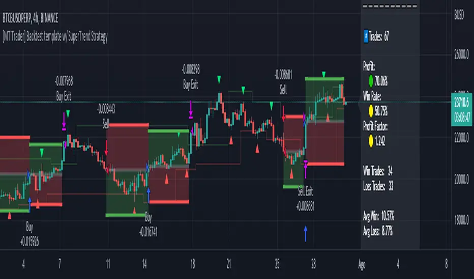
Simple RSI stock Strategy [1D] The "Simple RSI Stock Strategy " is designed to long-term traders. Strategy uses a daily time frame to capitalize on signals generated by the Relative Strength Index (RSI) and the Simple Moving Average (SMA). This strategy is suitable for low-leverage trading environments and focuses on identifying potential buy opportunities when the market is oversold, while incorporating strong risk management with both dynamic and static Stop Loss mechanisms.
This strategy is recommended for use with a relatively small amount of capital and is best applied by diversifying across multiple stocks in a strong uptrend, particularly in the S&P 500 stock market. It is specifically designed for equities, and may not perform well in other markets such as commodities, forex, or cryptocurrencies, where different market dynamics and volatility patterns apply.
Indicators Used in the Strategy:
1. RSI (Relative Strength Index):
- The RSI is a momentum oscillator used to identify overbought and oversold conditions in the market.
- This strategy enters long positions when the RSI drops below the oversold level (default: 30), indicating a potential buying opportunity.
- It focuses on oversold conditions but uses a filter (SMA 200) to ensure trades are only made in the context of an overall uptrend.
2. SMA 200 (Simple Moving Average):
- The 200-period SMA serves as a trend filter, ensuring that trades are only executed when the price is above the SMA, signaling a bullish market.
- This filter helps to avoid entering trades in a downtrend, thereby reducing the risk of holding positions in a declining market.
3. ATR (Average True Range):
- The ATR is used to measure market volatility and is instrumental in setting the Stop Loss.
- By multiplying the ATR value by a custom multiplier (default: 1.5), the strategy dynamically adjusts the Stop Loss level based on market volatility, allowing for flexibility in risk management.
How the Strategy Works:
Entry Signals:
The strategy opens long positions when RSI indicates that the market is oversold (below 30), and the price is above the 200-period SMA. This ensures that the strategy buys into potential market bottoms within the context of a long-term uptrend.
Take Profit Levels:
The strategy defines three distinct Take Profit (TP) levels:
TP 1: A 5% from the entry price.
TP 2: A 10% from the entry price.
TP 3: A 15% from the entry price.
As each TP level is reached, the strategy closes portions of the position to secure profits: 33% of the position is closed at TP 1, 66% at TP 2, and 100% at TP 3.
Visualizing Target Points:
The strategy provides visual feedback by plotting plotshapes at each Take Profit level (TP 1, TP 2, TP 3). This allows traders to easily see the target profit levels on the chart, making it easier to monitor and manage positions as they approach key profit-taking areas.
Stop Loss Mechanism:
The strategy uses a dual Stop Loss system to effectively manage risk:
ATR Trailing Stop: This dynamic Stop Loss adjusts based on the ATR value and trails the price as the position moves in the trader’s favor. If a price reversal occurs and the market begins to trend downward, the trailing stop closes the position, locking in gains or minimizing losses.
Basic Stop Loss: Additionally, a fixed Stop Loss is set at 25%, limiting potential losses. This basic Stop Loss serves as a safeguard, automatically closing the position if the price drops 25% from the entry point. This higher Stop Loss is designed specifically for low-leverage trading, allowing more room for market fluctuations without prematurely closing positions.
to determine the level of stop loss and target point I used a piece of code by RafaelZioni, here is the script from which a piece of code was taken
Together, these mechanisms ensure that the strategy dynamically manages risk while offering robust protection against significant losses in case of sharp market downturns.
The position size has been estimated by me at 75% of the total capital. For optimal capital allocation, a recommended value based on the Kelly Criterion, which is calculated to be 59.13% of the total capital per trade, can also be considered.
Enjoy !

Adaptive Market Wave TheoryAdaptive Market Wave Theory
🌊 CORE INNOVATION: PROBABILISTIC PHASE DETECTION WITH MULTI-AGENT CONSENSUS
Adaptive Market Wave Theory (AMWT) represents a fundamental paradigm shift in how traders approach market phase identification. Rather than counting waves subjectively or drawing static breakout levels, AMWT treats the market as a hidden state machine —using Hidden Markov Models, multi-agent consensus systems, and reinforcement learning algorithms to quantify what traditional methods leave to interpretation.
The Wave Analysis Problem:
Traditional wave counting methodologies (Elliott Wave, harmonic patterns, ABC corrections) share fatal weaknesses that AMWT directly addresses:
1. Non-Falsifiability : Invalid wave counts can always be "recounted" or "adjusted." If your Wave 3 fails, it becomes "Wave 3 of a larger degree" or "actually Wave C." There's no objective failure condition.
2. Observer Bias : Two expert wave analysts examining the same chart routinely reach different conclusions. This isn't a feature—it's a fundamental methodology flaw.
3. No Confidence Measure : Traditional analysis says "This IS Wave 3." But with what probability? 51%? 95%? The binary nature prevents proper position sizing and risk management.
4. Static Rules : Fixed Fibonacci ratios and wave guidelines cannot adapt to changing market regimes. What worked in 2019 may fail in 2024.
5. No Accountability : Wave methodologies rarely track their own performance. There's no feedback loop to improve.
The AMWT Solution:
AMWT addresses each limitation through rigorous mathematical frameworks borrowed from speech recognition, machine learning, and reinforcement learning:
• Non-Falsifiability → Hard Invalidation : Wave hypotheses die permanently when price violates calculated invalidation levels. No recounting allowed.
• Observer Bias → Multi-Agent Consensus : Three independent analytical agents must agree. Single-methodology bias is eliminated.
• No Confidence → Probabilistic States : Every market state has a calculated probability from Hidden Markov Model inference. "72% probability of impulse state" replaces "This is Wave 3."
• Static Rules → Adaptive Learning : Thompson Sampling multi-armed bandits learn which agents perform best in current conditions. The system adapts in real-time.
• No Accountability → Performance Tracking : Comprehensive statistics track every signal's outcome. The system knows its own performance.
The Core Insight:
"Traditional wave analysis asks 'What count is this?' AMWT asks 'What is the probability we are in an impulsive state, with what confidence, confirmed by how many independent methodologies, and anchored to what liquidity event?'"
🔬 THEORETICAL FOUNDATION: HIDDEN MARKOV MODELS
Why Hidden Markov Models?
Markets exist in hidden states that we cannot directly observe—only their effects on price are visible. When the market is in an "impulse up" state, we see rising prices, expanding volume, and trending indicators. But we don't observe the state itself—we infer it from observables.
This is precisely the problem Hidden Markov Models (HMMs) solve. Originally developed for speech recognition (inferring words from sound waves), HMMs excel at estimating hidden states from noisy observations.
HMM Components:
1. Hidden States (S) : The unobservable market conditions
2. Observations (O) : What we can measure (price, volume, indicators)
3. Transition Matrix (A) : Probability of moving between states
4. Emission Matrix (B) : Probability of observations given each state
5. Initial Distribution (π) : Starting state probabilities
AMWT's Six Market States:
State 0: IMPULSE_UP
• Definition: Strong bullish momentum with high participation
• Observable Signatures: Rising prices, expanding volume, RSI >60, price above upper Bollinger Band, MACD histogram positive and rising
• Typical Duration: 5-20 bars depending on timeframe
• What It Means: Institutional buying pressure, trend acceleration phase
State 1: IMPULSE_DN
• Definition: Strong bearish momentum with high participation
• Observable Signatures: Falling prices, expanding volume, RSI <40, price below lower Bollinger Band, MACD histogram negative and falling
• Typical Duration: 5-20 bars (often shorter than bullish impulses—markets fall faster)
• What It Means: Institutional selling pressure, panic or distribution acceleration
State 2: CORRECTION
• Definition: Counter-trend consolidation with declining momentum
• Observable Signatures: Sideways or mild counter-trend movement, contracting volume, RSI returning toward 50, Bollinger Bands narrowing
• Typical Duration: 8-30 bars
• What It Means: Profit-taking, digestion of prior move, potential accumulation for next leg
State 3: ACCUMULATION
• Definition: Base-building near lows where informed participants absorb supply
• Observable Signatures: Price near recent lows but not making new lows, volume spikes on up bars, RSI showing positive divergence, tight range
• Typical Duration: 15-50 bars
• What It Means: Smart money buying from weak hands, preparing for markup phase
State 4: DISTRIBUTION
• Definition: Top-forming near highs where informed participants distribute holdings
• Observable Signatures: Price near recent highs but struggling to advance, volume spikes on down bars, RSI showing negative divergence, widening range
• Typical Duration: 15-50 bars
• What It Means: Smart money selling to late buyers, preparing for markdown phase
State 5: TRANSITION
• Definition: Regime change period with mixed signals and elevated uncertainty
• Observable Signatures: Conflicting indicators, whipsaw price action, no clear momentum, high volatility without direction
• Typical Duration: 5-15 bars
• What It Means: Market deciding next direction, dangerous for directional trades
The Transition Matrix:
The transition matrix A captures the probability of moving from one state to another. AMWT initializes with empirically-derived values then updates online:
From/To IMP_UP IMP_DN CORR ACCUM DIST TRANS
IMP_UP 0.70 0.02 0.20 0.02 0.04 0.02
IMP_DN 0.02 0.70 0.20 0.04 0.02 0.02
CORR 0.15 0.15 0.50 0.10 0.10 0.00
ACCUM 0.30 0.05 0.15 0.40 0.05 0.05
DIST 0.05 0.30 0.15 0.05 0.40 0.05
TRANS 0.20 0.20 0.20 0.15 0.15 0.10
Key Insights from Transition Probabilities:
• Impulse states are sticky (70% self-transition): Once trending, markets tend to continue
• Corrections can transition to either impulse direction (15% each): The next move after correction is uncertain
• Accumulation strongly favors IMP_UP transition (30%): Base-building leads to rallies
• Distribution strongly favors IMP_DN transition (30%): Topping leads to declines
The Viterbi Algorithm:
Given a sequence of observations, how do we find the most likely state sequence? This is the Viterbi algorithm—dynamic programming to find the optimal path through the state space.
Mathematical Formulation:
δ_t(j) = max_i × B_j(O_t)
Where:
δ_t(j) = probability of most likely path ending in state j at time t
A_ij = transition probability from state i to state j
B_j(O_t) = emission probability of observation O_t given state j
AMWT Implementation:
AMWT runs Viterbi over a rolling window (default 50 bars), computing the most likely state sequence and extracting:
• Current state estimate
• State confidence (probability of current state vs alternatives)
• State sequence for pattern detection
Online Learning (Baum-Welch Adaptation):
Unlike static HMMs, AMWT continuously updates its transition and emission matrices based on observed market behavior:
f_onlineUpdateHMM(prev_state, curr_state, observation, decay) =>
// Update transition matrix
A *= decay
A += (1.0 - decay)
// Renormalize row
// Update emission matrix
B *= decay
B += (1.0 - decay)
// Renormalize row
The decay parameter (default 0.85) controls adaptation speed:
• Higher decay (0.95): Slower adaptation, more stable, better for consistent markets
• Lower decay (0.80): Faster adaptation, more reactive, better for regime changes
Why This Matters for Trading:
Traditional indicators give you a number (RSI = 72). AMWT gives you a probabilistic state assessment :
"There is a 78% probability we are in IMPULSE_UP state, with 15% probability of CORRECTION and 7% distributed among other states. The transition matrix suggests 70% chance of remaining in IMPULSE_UP next bar, 20% chance of transitioning to CORRECTION."
This enables:
• Position sizing by confidence : 90% confidence = full size; 60% confidence = half size
• Risk management by transition probability : High correction probability = tighten stops
• Strategy selection by state : IMPULSE = trend-follow; CORRECTION = wait; ACCUMULATION = scale in
🎰 THE 3-BANDIT CONSENSUS SYSTEM
The Multi-Agent Philosophy:
No single analytical methodology works in all market conditions. Trend-following excels in trending markets but gets chopped in ranges. Mean-reversion excels in ranges but gets crushed in trends. Structure-based analysis works when structure is clear but fails in chaotic markets.
AMWT's solution: employ three independent agents , each analyzing the market from a different perspective, then use Thompson Sampling to learn which agents perform best in current conditions.
Agent 1: TREND AGENT
Philosophy : Markets trend. Follow the trend until it ends.
Analytical Components:
• EMA Alignment: EMA8 > EMA21 > EMA50 (bullish) or inverse (bearish)
• MACD Histogram: Direction and rate of change
• Price Momentum: Close relative to ATR-normalized movement
• VWAP Position: Price above/below volume-weighted average price
Signal Generation:
Strong Bull: EMA aligned bull AND MACD histogram > 0 AND momentum > 0.3 AND close > VWAP
→ Signal: +1 (Long), Confidence: 0.75 + |momentum| × 0.4
Moderate Bull: EMA stack bull AND MACD rising AND momentum > 0.1
→ Signal: +1 (Long), Confidence: 0.65 + |momentum| × 0.3
Strong Bear: EMA aligned bear AND MACD histogram < 0 AND momentum < -0.3 AND close < VWAP
→ Signal: -1 (Short), Confidence: 0.75 + |momentum| × 0.4
Moderate Bear: EMA stack bear AND MACD falling AND momentum < -0.1
→ Signal: -1 (Short), Confidence: 0.65 + |momentum| × 0.3
When Trend Agent Excels:
• Trend days (IB extension >1.5x)
• Post-breakout continuation
• Institutional accumulation/distribution phases
When Trend Agent Fails:
• Range-bound markets (ADX <20)
• Chop zones after volatility spikes
• Reversal days at major levels
Agent 2: REVERSION AGENT
Philosophy: Markets revert to mean. Extreme readings reverse.
Analytical Components:
• Bollinger Band Position: Distance from bands, percent B
• RSI Extremes: Overbought (>70) and oversold (<30)
• Stochastic: %K/%D crossovers at extremes
• Band Squeeze: Bollinger Band width contraction
Signal Generation:
Oversold Bounce: BB %B < 0.20 AND RSI < 35 AND Stochastic < 25
→ Signal: +1 (Long), Confidence: 0.70 + (30 - RSI) × 0.01
Overbought Fade: BB %B > 0.80 AND RSI > 65 AND Stochastic > 75
→ Signal: -1 (Short), Confidence: 0.70 + (RSI - 70) × 0.01
Squeeze Fire Bull: Band squeeze ending AND close > upper band
→ Signal: +1 (Long), Confidence: 0.65
Squeeze Fire Bear: Band squeeze ending AND close < lower band
→ Signal: -1 (Short), Confidence: 0.65
When Reversion Agent Excels:
• Rotation days (price stays within IB)
• Range-bound consolidation
• After extended moves without pullback
When Reversion Agent Fails:
• Strong trend days (RSI can stay overbought for days)
• Breakout moves
• News-driven directional moves
Agent 3: STRUCTURE AGENT
Philosophy: Market structure reveals institutional intent. Follow the smart money.
Analytical Components:
• Break of Structure (BOS): Price breaks prior swing high/low
• Change of Character (CHOCH): First break against prevailing trend
• Higher Highs/Higher Lows: Bullish structure
• Lower Highs/Lower Lows: Bearish structure
• Liquidity Sweeps: Stop runs that reverse
Signal Generation:
BOS Bull: Price breaks above prior swing high with momentum
→ Signal: +1 (Long), Confidence: 0.70 + structure_strength × 0.2
CHOCH Bull: First higher low after downtrend, breaking structure
→ Signal: +1 (Long), Confidence: 0.75
BOS Bear: Price breaks below prior swing low with momentum
→ Signal: -1 (Short), Confidence: 0.70 + structure_strength × 0.2
CHOCH Bear: First lower high after uptrend, breaking structure
→ Signal: -1 (Short), Confidence: 0.75
Liquidity Sweep Long: Price sweeps below swing low then reverses strongly
→ Signal: +1 (Long), Confidence: 0.80
Liquidity Sweep Short: Price sweeps above swing high then reverses strongly
→ Signal: -1 (Short), Confidence: 0.80
When Structure Agent Excels:
• After liquidity grabs (stop runs)
• At major swing points
• During institutional accumulation/distribution
When Structure Agent Fails:
• Choppy, structureless markets
• During news events (structure becomes noise)
• Very low timeframes (noise overwhelms structure)
Thompson Sampling: The Bandit Algorithm
With three agents giving potentially different signals, how do we decide which to trust? This is the multi-armed bandit problem —balancing exploitation (using what works) with exploration (testing alternatives).
Thompson Sampling Solution:
Each agent maintains a Beta distribution representing its success/failure history:
Agent success rate modeled as Beta(α, β)
Where:
α = number of successful signals + 1
β = number of failed signals + 1
On Each Bar:
1. Sample from each agent's Beta distribution
2. Weight agent signals by sampled probabilities
3. Combine weighted signals into consensus
4. Update α/β based on trade outcomes
Mathematical Implementation:
// Beta sampling via Gamma ratio method
f_beta_sample(alpha, beta) =>
g1 = f_gamma_sample(alpha)
g2 = f_gamma_sample(beta)
g1 / (g1 + g2)
// Thompson Sampling selection
for each agent:
sampled_prob = f_beta_sample(agent.alpha, agent.beta)
weight = sampled_prob / sum(all_sampled_probs)
consensus += agent.signal × agent.confidence × weight
Why Thompson Sampling?
• Automatic Exploration : Agents with few samples get occasional chances (high variance in Beta distribution)
• Bayesian Optimal : Mathematically proven optimal solution to exploration-exploitation tradeoff
• Uncertainty-Aware : Small sample size = more exploration; large sample size = more exploitation
• Self-Correcting : Poor performers naturally get lower weights over time
Example Evolution:
Day 1 (Initial):
Trend Agent: Beta(1,1) → samples ~0.50 (high uncertainty)
Reversion Agent: Beta(1,1) → samples ~0.50 (high uncertainty)
Structure Agent: Beta(1,1) → samples ~0.50 (high uncertainty)
After 50 Signals:
Trend Agent: Beta(28,23) → samples ~0.55 (moderate confidence)
Reversion Agent: Beta(18,33) → samples ~0.35 (underperforming)
Structure Agent: Beta(32,19) → samples ~0.63 (outperforming)
Result: Structure Agent now receives highest weight in consensus
Consensus Requirements by Mode:
Aggressive Mode:
• Minimum 1/3 agents agreeing
• Consensus threshold: 45%
• Use case: More signals, higher risk tolerance
Balanced Mode:
• Minimum 2/3 agents agreeing
• Consensus threshold: 55%
• Use case: Standard trading
Conservative Mode:
• Minimum 2/3 agents agreeing
• Consensus threshold: 65%
• Use case: Higher quality, fewer signals
Institutional Mode:
• Minimum 2/3 agents agreeing
• Consensus threshold: 75%
• Additional: Session quality >0.65, mode adjustment +0.10
• Use case: Highest quality signals only
🌀 INTELLIGENT CHOP DETECTION ENGINE
The Chop Problem:
Most trading losses occur not from being wrong about direction, but from trading in conditions where direction doesn't exist . Choppy, range-bound markets generate false signals from every methodology—trend-following, mean-reversion, and structure-based alike.
AMWT's chop detection engine identifies these low-probability environments before signals fire, preventing the most damaging trades.
Five-Factor Chop Analysis:
Factor 1: ADX Component (25% weight)
ADX (Average Directional Index) measures trend strength regardless of direction.
ADX < 15: Very weak trend (high chop score)
ADX 15-20: Weak trend (moderate chop score)
ADX 20-25: Developing trend (low chop score)
ADX > 25: Strong trend (minimal chop score)
adx_chop = (i_adxThreshold - adx_val) / i_adxThreshold × 100
Why ADX Works: ADX synthesizes +DI and -DI movements. Low ADX means price is moving but not directionally—the definition of chop.
Factor 2: Choppiness Index (25% weight)
The Choppiness Index measures price efficiency using the ratio of ATR sum to price range:
CI = 100 × LOG10(SUM(ATR, n) / (Highest - Lowest)) / LOG10(n)
CI > 61.8: Choppy (range-bound, inefficient movement)
CI < 38.2: Trending (directional, efficient movement)
CI 38.2-61.8: Transitional
chop_idx_score = (ci_val - 38.2) / (61.8 - 38.2) × 100
Why Choppiness Index Works: In trending markets, price covers distance efficiently (low ATR sum relative to range). In choppy markets, price oscillates wildly but goes nowhere (high ATR sum relative to range).
Factor 3: Range Compression (20% weight)
Compares recent range to longer-term range, detecting volatility squeezes:
recent_range = Highest(20) - Lowest(20)
longer_range = Highest(50) - Lowest(50)
compression = 1 - (recent_range / longer_range)
compression > 0.5: Strong squeeze (potential breakout imminent)
compression < 0.2: No compression (normal volatility)
range_compression_score = compression × 100
Why Range Compression Matters: Compression precedes expansion. High compression = market coiling, preparing for move. Signals during compression often fail because the breakout hasn't occurred yet.
Factor 4: Channel Position (15% weight)
Tracks price position within the macro channel:
channel_position = (close - channel_low) / (channel_high - channel_low)
position 0.4-0.6: Center of channel (indecision zone)
position <0.2 or >0.8: Near extremes (potential reversal or breakout)
channel_chop = abs(0.5 - channel_position) < 0.15 ? high_score : low_score
Why Channel Position Matters: Price in the middle of a range is in "no man's land"—equally likely to go either direction. Signals in the channel center have lower probability.
Factor 5: Volume Quality (15% weight)
Assesses volume relative to average:
vol_ratio = volume / SMA(volume, 20)
vol_ratio < 0.7: Low volume (lack of conviction)
vol_ratio 0.7-1.3: Normal volume
vol_ratio > 1.3: High volume (conviction present)
volume_chop = vol_ratio < 0.8 ? (1 - vol_ratio) × 100 : 0
Why Volume Quality Matters: Low volume moves lack institutional participation. These moves are more likely to reverse or stall.
Combined Chop Intensity:
chopIntensity = (adx_chop × 0.25) + (chop_idx_score × 0.25) +
(range_compression_score × 0.20) + (channel_chop × 0.15) +
(volume_chop × i_volumeChopWeight × 0.15)
Regime Classifications:
Based on chop intensity and component analysis:
• Strong Trend (0-20%): ADX >30, clear directional momentum, trade aggressively
• Trending (20-35%): ADX >20, moderate directional bias, trade normally
• Transitioning (35-50%): Mixed signals, regime change possible, reduce size
• Mid-Range (50-60%): Price trapped in channel center, avoid new positions
• Ranging (60-70%): Low ADX, price oscillating within bounds, fade extremes only
• Compression (70-80%): Volatility squeeze, expansion imminent, wait for breakout
• Strong Chop (80-100%): Multiple chop factors aligned, avoid trading entirely
Signal Suppression:
When chop intensity exceeds the configurable threshold (default 80%), signals are suppressed entirely. The dashboard displays "⚠️ CHOP ZONE" with the current regime classification.
Chop Box Visualization:
When chop is detected, AMWT draws a semi-transparent box on the chart showing the chop zone. This visual reminder helps traders avoid entering positions during unfavorable conditions.
💧 LIQUIDITY ANCHORING SYSTEM
The Liquidity Concept:
Markets move from liquidity pool to liquidity pool. Stop losses cluster at predictable locations—below swing lows (buy stops become sell orders when triggered) and above swing highs (sell stops become buy orders when triggered). Institutions know where these clusters are and often engineer moves to trigger them before reversing.
AMWT identifies and tracks these liquidity events, using them as anchors for signal confidence.
Liquidity Event Types:
Type 1: Volume Spikes
Definition: Volume > SMA(volume, 20) × i_volThreshold (default 2.8x)
Interpretation: Sudden volume surge indicates institutional activity
• Near swing low + reversal: Likely accumulation
• Near swing high + reversal: Likely distribution
• With continuation: Institutional conviction in direction
Type 2: Stop Runs (Liquidity Sweeps)
Definition: Price briefly exceeds swing high/low then reverses within N bars
Detection:
• Price breaks above recent swing high (triggering buy stops)
• Then closes back below that high within 3 bars
• Signal: Bullish stop run complete, reversal likely
Or inverse for bearish:
• Price breaks below recent swing low (triggering sell stops)
• Then closes back above that low within 3 bars
• Signal: Bearish stop run complete, reversal likely
Type 3: Absorption Events
Definition: High volume with small candle body
Detection:
• Volume > 2x average
• Candle body < 30% of candle range
• Interpretation: Large orders being filled without moving price
• Implication: Accumulation (at lows) or distribution (at highs)
Type 4: BSL/SSL Pools (Buy-Side/Sell-Side Liquidity)
BSL (Buy-Side Liquidity):
• Cluster of swing highs within ATR proximity
• Stop losses from shorts sit above these highs
• Breaking BSL triggers short covering (fuel for rally)
SSL (Sell-Side Liquidity):
• Cluster of swing lows within ATR proximity
• Stop losses from longs sit below these lows
• Breaking SSL triggers long liquidation (fuel for decline)
Liquidity Pool Mapping:
AMWT continuously scans for and maps liquidity pools:
// Detect swing highs/lows using pivot function
swing_high = ta.pivothigh(high, 5, 5)
swing_low = ta.pivotlow(low, 5, 5)
// Track recent swing points
if not na(swing_high)
bsl_levels.push(swing_high)
if not na(swing_low)
ssl_levels.push(swing_low)
// Display on chart with labels
Confluence Scoring Integration:
When signals fire near identified liquidity events, confluence scoring increases:
• Signal near volume spike: +10% confidence
• Signal after liquidity sweep: +15% confidence
• Signal at BSL/SSL pool: +10% confidence
• Signal aligned with absorption zone: +10% confidence
Why Liquidity Anchoring Matters:
Signals "in a vacuum" have lower probability than signals anchored to institutional activity. A long signal after a liquidity sweep below swing lows has trapped shorts providing fuel. A long signal in the middle of nowhere has no such catalyst.
📊 SIGNAL GRADING SYSTEM
The Quality Problem:
Not all signals are created equal. A signal with 6/6 factors aligned is fundamentally different from a signal with 3/6 factors aligned. Traditional indicators treat them the same. AMWT grades every signal based on confluence.
Confluence Components (100 points total):
1. Bandit Consensus Strength (25 points)
consensus_str = weighted average of agent confidences
score = consensus_str × 25
Example:
Trend Agent: +1 signal, 0.80 confidence, 0.35 weight
Reversion Agent: 0 signal, 0.50 confidence, 0.25 weight
Structure Agent: +1 signal, 0.75 confidence, 0.40 weight
Weighted consensus = (0.80×0.35 + 0×0.25 + 0.75×0.40) / (0.35 + 0.40) = 0.77
Score = 0.77 × 25 = 19.25 points
2. HMM State Confidence (15 points)
score = hmm_confidence × 15
Example:
HMM reports 82% probability of IMPULSE_UP
Score = 0.82 × 15 = 12.3 points
3. Session Quality (15 points)
Session quality varies by time:
• London/NY Overlap: 1.0 (15 points)
• New York Session: 0.95 (14.25 points)
• London Session: 0.70 (10.5 points)
• Asian Session: 0.40 (6 points)
• Off-Hours: 0.30 (4.5 points)
• Weekend: 0.10 (1.5 points)
4. Energy/Participation (10 points)
energy = (realized_vol / avg_vol) × 0.4 + (range / ATR) × 0.35 + (volume / avg_volume) × 0.25
score = min(energy, 1.0) × 10
5. Volume Confirmation (10 points)
if volume > SMA(volume, 20) × 1.5:
score = 10
else if volume > SMA(volume, 20):
score = 5
else:
score = 0
6. Structure Alignment (10 points)
For long signals:
• Bullish structure (HH + HL): 10 points
• Higher low only: 6 points
• Neutral structure: 3 points
• Bearish structure: 0 points
Inverse for short signals
7. Trend Alignment (10 points)
For long signals:
• Price > EMA21 > EMA50: 10 points
• Price > EMA21: 6 points
• Neutral: 3 points
• Against trend: 0 points
8. Entry Trigger Quality (5 points)
• Strong trigger (multiple confirmations): 5 points
• Moderate trigger (single confirmation): 3 points
• Weak trigger (marginal): 1 point
Grade Scale:
Total Score → Grade
85-100 → A+ (Exceptional—all factors aligned)
70-84 → A (Strong—high probability)
55-69 → B (Acceptable—proceed with caution)
Below 55 → C (Marginal—filtered by default)
Grade-Based Signal Brightness:
Signal arrows on the chart have transparency based on grade:
• A+: Full brightness (alpha = 0)
• A: Slight fade (alpha = 15)
• B: Moderate fade (alpha = 35)
• C: Significant fade (alpha = 55)
This visual hierarchy helps traders instantly identify signal quality.
Minimum Grade Filter:
Configurable filter (default: C) sets the minimum grade for signal display:
• Set to "A" for only highest-quality signals
• Set to "B" for moderate selectivity
• Set to "C" for all signals (maximum quantity)
🕐 SESSION INTELLIGENCE
Why Sessions Matter:
Markets behave differently at different times. The London open is fundamentally different from the Asian lunch hour. AMWT incorporates session-aware logic to optimize signal quality.
Session Definitions:
Asian Session (18:00-03:00 ET)
• Characteristics: Lower volatility, range-bound tendency, fewer institutional participants
• Quality Score: 0.40 (40% of peak quality)
• Strategy Implications: Fade extremes, expect ranges, smaller position sizes
• Best For: Mean-reversion setups, accumulation/distribution identification
London Session (03:00-12:00 ET)
• Characteristics: European institutional activity, volatility pickup, trend initiation
• Quality Score: 0.70 (70% of peak quality)
• Strategy Implications: Watch for trend development, breakouts more reliable
• Best For: Initial trend identification, structure breaks
New York Session (08:00-17:00 ET)
• Characteristics: Highest liquidity, US institutional activity, major moves
• Quality Score: 0.95 (95% of peak quality)
• Strategy Implications: Best environment for directional trades
• Best For: Trend continuation, momentum plays
London/NY Overlap (08:00-12:00 ET)
• Characteristics: Peak liquidity, both European and US participants active
• Quality Score: 1.0 (100%—maximum quality)
• Strategy Implications: Highest probability for successful breakouts and trends
• Best For: All signal types—this is prime time
Off-Hours
• Characteristics: Thin liquidity, erratic price action, gaps possible
• Quality Score: 0.30 (30% of peak quality)
• Strategy Implications: Avoid new positions, wider stops if holding
• Best For: Waiting
Smart Weekend Detection:
AMWT properly handles the Sunday evening futures open:
// Traditional (broken):
isWeekend = dayofweek == saturday OR dayofweek == sunday
// AMWT (correct):
anySessionActive = not na(asianTime) or not na(londonTime) or not na(nyTime)
isWeekend = calendarWeekend AND NOT anySessionActive
This ensures Sunday 6pm ET (when futures open) correctly shows "Asian Session" rather than "Weekend."
Session Transition Boosts:
Certain session transitions create trading opportunities:
• Asian → London transition: +15% confidence boost (volatility expansion likely)
• London → Overlap transition: +20% confidence boost (peak liquidity approaching)
• Overlap → NY-only transition: -10% confidence adjustment (liquidity declining)
• Any → Off-Hours transition: Signal suppression recommended
📈 TRADE MANAGEMENT SYSTEM
The Signal Spam Problem:
Many indicators generate signal after signal, creating confusion and overtrading. AMWT implements a complete trade lifecycle management system that prevents signal spam and tracks performance.
Trade Lock Mechanism:
Once a signal fires, the system enters a "trade lock" state:
Trade Lock Duration: Configurable (default 30 bars)
Early Exit Conditions:
• TP3 hit (full target reached)
• Stop Loss hit (trade failed)
• Lock expiration (time-based exit)
During lock:
• No new signals of same type displayed
• Opposite signals can override (reversal)
• Trade status tracked in dashboard
Target Levels:
Each signal generates three profit targets based on ATR:
TP1 (Conservative Target)
• Default: 1.0 × ATR
• Purpose: Quick partial profit, reduce risk
• Action: Take 30-40% off position, move stop to breakeven
TP2 (Standard Target)
• Default: 2.5 × ATR
• Purpose: Main profit target
• Action: Take 40-50% off position, trail stop
TP3 (Extended Target)
• Default: 5.0 × ATR
• Purpose: Runner target for trend days
• Action: Close remaining position or continue trailing
Stop Loss:
• Default: 1.9 × ATR from entry
• Purpose: Define maximum risk
• Placement: Below recent swing low (longs) or above recent swing high (shorts)
Invalidation Level:
Beyond stop loss, AMWT calculates an "invalidation" level where the wave hypothesis dies:
invalidation = entry - (ATR × INVALIDATION_MULT × 1.5)
If price reaches invalidation, the current market interpretation is wrong—not just the trade.
Visual Trade Management:
During active trades, AMWT displays:
• Entry arrow with grade label (▲A+, ▼B, etc.)
• TP1, TP2, TP3 horizontal lines in green
• Stop Loss line in red
• Invalidation line in orange (dashed)
• Progress indicator in dashboard
Persistent Execution Markers:
When targets or stops are hit, permanent markers appear:
• TP hit: Green dot with "TP1"/"TP2"/"TP3" label
• SL hit: Red dot with "SL" label
These persist on the chart for review and statistics.
💰 PERFORMANCE TRACKING & STATISTICS
Tracked Metrics:
• Total Trades: Count of all signals that entered trade lock
• Winning Trades: Signals where at least TP1 was reached before SL
• Losing Trades: Signals where SL was hit before any TP
• Win Rate: Winning / Total × 100%
• Total R Profit: Sum of R-multiples from winning trades
• Total R Loss: Sum of R-multiples from losing trades
• Net R: Total R Profit - Total R Loss
Currency Conversion System:
AMWT can display P&L in multiple formats:
R-Multiple (Default)
• Shows risk-normalized returns
• "Net P&L: +4.2R | 78 trades" means 4.2 times initial risk gained over 78 trades
• Best for comparing across different position sizes
Currency Conversion (USD/EUR/GBP/JPY/INR)
• Converts R-multiples to currency based on:
- Dollar Risk Per Trade (user input)
- Tick Value (user input)
- Selected currency
Example Configuration:
Dollar Risk Per Trade: $100
Display Currency: USD
If Net R = +4.2R
Display: Net P&L: +$420.00 | 78 trades
Ticks
• For futures traders who think in ticks
• Converts based on tick value input
Statistics Reset:
Two reset methods:
1. Toggle Reset
• Turn "Reset Statistics" toggle ON then OFF
• Clears all statistics immediately
2. Date-Based Reset
• Set "Reset After Date" (YYYY-MM-DD format)
• Only trades after this date are counted
• Useful for isolating recent performance
🎨 VISUAL FEATURES
Macro Channel:
Dynamic regression-based channel showing market boundaries:
• Upper/lower bounds calculated from swing pivot linear regression
• Adapts to current market structure
• Shows overall trend direction and potential reversal zones
Chop Boxes:
Semi-transparent overlay during high-chop periods:
• Purple/orange coloring indicates dangerous conditions
• Visual reminder to avoid new positions
Confluence Heat Zones:
Background shading indicating setup quality:
• Darker shading = higher confluence
• Lighter shading = lower confluence
• Helps identify optimal entry timing
EMA Ribbon:
Trend visualization via moving average fill:
• EMA 8/21/50 with gradient fill between
• Green fill when bullish aligned
• Red fill when bearish aligned
• Gray when neutral
Absorption Zone Boxes:
Marks potential accumulation/distribution areas:
• High volume + small body = absorption
• Boxes drawn at these levels
• Often act as support/resistance
Liquidity Pool Lines:
BSL/SSL levels with labels:
• Dashed lines at liquidity clusters
• "BSL" label above swing high clusters
• "SSL" label below swing low clusters
Six Professional Themes:
• Quantum: Deep purples and cyans (default)
• Cyberpunk: Neon pinks and blues
• Professional: Muted grays and greens
• Ocean: Blues and teals
• Matrix: Greens and blacks
• Ember: Oranges and reds
🎓 PROFESSIONAL USAGE PROTOCOL
Phase 1: Learning the System (Week 1)
Goal: Understand AMWT concepts and dashboard interpretation
Setup:
• Signal Mode: Balanced
• Display: All features enabled
• Grade Filter: C (see all signals)
Actions:
• Paper trade ONLY—no real money
• Observe HMM state transitions throughout the day
• Note when agents agree vs disagree
• Watch chop detection engage and disengage
• Track which grades produce winners vs losers
Key Learning Questions:
• How often do A+ signals win vs B signals? (Should see clear difference)
• Which agent tends to be right in current market? (Check dashboard)
• When does chop detection save you from bad trades?
• How do signals near liquidity events perform vs signals in vacuum?
Phase 2: Parameter Optimization (Week 2)
Goal: Tune system to your instrument and timeframe
Signal Mode Testing:
• Run 5 days on Aggressive mode (more signals)
• Run 5 days on Conservative mode (fewer signals)
• Compare: Which produces better risk-adjusted returns?
Grade Filter Testing:
• Track A+ only for 20 signals
• Track A and above for 20 signals
• Track B and above for 20 signals
• Compare win rates and expectancy
Chop Threshold Testing:
• Default (80%): Standard filtering
• Try 70%: More aggressive filtering
• Try 90%: Less filtering
• Which produces best results for your instrument?
Phase 3: Strategy Development (Weeks 3-4)
Goal: Develop personal trading rules based on system signals
Position Sizing by Grade:
• A+ grade: 100% position size
• A grade: 75% position size
• B grade: 50% position size
• C grade: 25% position size (or skip)
Session-Based Rules:
• London/NY Overlap: Take all A/A+ signals
• NY Session: Take all A+ signals, selective on A
• Asian Session: Only A+ signals with extra confirmation
• Off-Hours: No new positions
Chop Zone Rules:
• Chop >70%: Reduce position size 50%
• Chop >80%: No new positions
• Chop <50%: Full position size allowed
Phase 4: Live Micro-Sizing (Month 2)
Goal: Validate paper trading results with minimal risk
Setup:
• 10-20% of intended full position size
• Take ONLY A+ signals initially
• Follow trade management religiously
Tracking:
• Log every trade: Entry, Exit, Grade, HMM State, Chop Level, Agent Consensus
• Calculate: Win rate by grade, by session, by chop level
• Compare to paper trading (should be within 15%)
Red Flags:
• Win rate diverges significantly from paper trading: Execution issues
• Consistent losses during certain sessions: Adjust session rules
• Losses cluster when specific agent dominates: Review that agent's logic
Phase 5: Scaling Up (Months 3-6)
Goal: Gradually increase to full position size
Progression:
• Month 3: 25-40% size (if micro-sizing profitable)
• Month 4: 40-60% size
• Month 5: 60-80% size
• Month 6: 80-100% size
Scale-Up Requirements:
• Minimum 30 trades at current size
• Win rate ≥50%
• Net R positive
• No revenge trading incidents
• Emotional control maintained
💡 DEVELOPMENT INSIGHTS
Why HMM Over Simple Indicators:
Early versions used standard indicators (RSI >70 = overbought, etc.). Win rates hovered at 52-55%. The problem: indicators don't capture state. RSI can stay "overbought" for weeks in a strong trend.
The insight: markets exist in states, and state persistence matters more than indicator levels. Implementing HMM with state transition probabilities increased signal quality significantly. The system now knows not just "RSI is high" but "we're in IMPULSE_UP state with 70% probability of staying in IMPULSE_UP."
The Multi-Agent Evolution:
Original version used a single analytical methodology—trend-following. Performance was inconsistent: great in trends, destroyed in ranges. Added mean-reversion agent: now it was inconsistent the other way.
The breakthrough: use multiple agents and let the system learn which works . Thompson Sampling wasn't the first attempt—tried simple averaging, voting, even hard-coded regime switching. Thompson Sampling won because it's mathematically optimal and automatically adapts without manual regime detection.
Chop Detection Revelation:
Chop detection was added almost as an afterthought. "Let's filter out obviously bad conditions." Testing revealed it was the most impactful single feature. Filtering chop zones reduced losing trades by 35% while only reducing total signals by 20%. The insight: avoiding bad trades matters more than finding good ones.
Liquidity Anchoring Discovery:
Watched hundreds of trades. Noticed pattern: signals that fired after liquidity events (stop runs, volume spikes) had significantly higher win rates than signals in quiet markets. Implemented liquidity detection and anchoring. Win rate on liquidity-anchored signals: 68% vs 52% on non-anchored signals.
The Grade System Impact:
Early system had binary signals (fire or don't fire). Adding grading transformed it. Traders could finally match position size to signal quality. A+ signals deserved full size; C signals deserved caution. Just implementing grade-based sizing improved portfolio Sharpe ratio by 0.3.
🚨 LIMITATIONS & CRITICAL ASSUMPTIONS
What AMWT Is NOT:
• NOT a Holy Grail : No system wins every trade. AMWT improves probability, not certainty.
• NOT Fully Automated : AMWT provides signals and analysis; execution requires human judgment.
• NOT News-Proof : Exogenous shocks (FOMC surprises, geopolitical events) invalidate all technical analysis.
• NOT for Scalping : HMM state estimation needs time to develop. Sub-minute timeframes are not appropriate.
Core Assumptions:
1. Markets Have States : Assumes markets transition between identifiable regimes. Violation: Random walk markets with no regime structure.
2. States Are Inferable : Assumes observable indicators reveal hidden states. Violation: Market manipulation creating false signals.
3. History Informs Future : Assumes past agent performance predicts future performance. Violation: Regime changes that invalidate historical patterns.
4. Liquidity Events Matter : Assumes institutional activity creates predictable patterns. Violation: Markets with no institutional participation.
Performs Best On:
• Liquid Futures : ES, NQ, MNQ, MES, CL, GC
• Major Forex Pairs : EUR/USD, GBP/USD, USD/JPY
• Large-Cap Stocks : AAPL, MSFT, TSLA, NVDA (>$5B market cap)
• Liquid Crypto : BTC, ETH on major exchanges
Performs Poorly On:
• Illiquid Instruments : Low volume stocks, exotic pairs
• Very Low Timeframes : Sub-5-minute charts (noise overwhelms signal)
• Binary Event Days : Earnings, FDA approvals, court rulings
• Manipulated Markets : Penny stocks, low-cap altcoins
Known Weaknesses:
• Warmup Period : HMM needs ~50 bars to initialize properly. Early signals may be unreliable.
• Regime Change Lag : Thompson Sampling adapts over time, not instantly. Sudden regime changes may cause short-term underperformance.
• Complexity : More parameters than simple indicators. Requires understanding to use effectively.
⚠️ RISK DISCLOSURE
Trading futures, stocks, options, forex, and cryptocurrencies involves substantial risk of loss and is not suitable for all investors. Adaptive Market Wave Theory, while based on rigorous mathematical frameworks including Hidden Markov Models and multi-armed bandit algorithms, does not guarantee profits and can result in significant losses.
AMWT's methodologies—HMM state estimation, Thompson Sampling agent selection, and confluence-based grading—have theoretical foundations but past performance is not indicative of future results.
Hidden Markov Model assumptions may not hold during:
• Major news events disrupting normal market behavior
• Flash crashes or circuit breaker events
• Low liquidity periods with erratic price action
• Algorithmic manipulation or spoofing
Multi-agent consensus assumes independent analytical perspectives provide edge. Market conditions change. Edges that existed historically can diminish or disappear.
Users must independently validate system performance on their specific instruments, timeframes, and broker execution environment. Paper trade extensively before risking capital. Start with micro position sizing.
Never risk more than you can afford to lose completely. Use proper position sizing. Implement stop losses without exception.
By using this indicator, you acknowledge these risks and accept full responsibility for all trading decisions and outcomes.
"Elliott Wave was a first-order approximation of market phase behavior. AMWT is the second—probabilistic, adaptive, and accountable."
Initial Public Release
Core Engine:
• True Hidden Markov Model with online Baum-Welch learning
• Viterbi algorithm for optimal state sequence decoding
• 6-state market regime classification
Agent System:
• 3-Bandit consensus (Trend, Reversion, Structure)
• Thompson Sampling with true Beta distribution sampling
• Adaptive weight learning based on performance
Signal Generation:
• Quality-based confluence grading (A+/A/B/C)
• Four signal modes (Aggressive/Balanced/Conservative/Institutional)
• Grade-based visual brightness
Chop Detection:
• 5-factor analysis (ADX, Choppiness Index, Range Compression, Channel Position, Volume)
• 7 regime classifications
• Configurable signal suppression threshold
Liquidity:
• Volume spike detection
• Stop run (liquidity sweep) identification
• BSL/SSL pool mapping
• Absorption zone detection
Trade Management:
• Trade lock with configurable duration
• TP1/TP2/TP3 targets
• ATR-based stop loss
• Persistent execution markers
Session Intelligence:
• Asian/London/NY/Overlap detection
• Smart weekend handling (Sunday futures open)
• Session quality scoring
Performance:
• Statistics tracking with reset functionality
• 7 currency display modes
• Win rate and Net R calculation
Visuals:
• Macro channel with linear regression
• Chop boxes
• EMA ribbon
• Liquidity pool lines
• 6 professional themes
Dashboards:
• Main Dashboard: Market State, Consensus, Trade Status, Statistics
📋 AMWT vs AMWT-PRO:
This version includes all core AMWT functionality:
✓ Full Hidden Markov Model state estimation
✓ 3-Bandit Thompson Sampling consensus system
✓ Complete 5-factor chop detection engine
✓ All four signal modes
✓ Full trade management with TP/SL tracking
✓ Main dashboard with complete statistics
✓ All visual features (channels, zones, pools)
✓ Identical signal generation to PRO
✓ Six professional themes
✓ Full alert system
The PRO version adds the AMWT Advisor panel—a secondary dashboard providing:
• Real-time Market Pulse situation assessment
• Agent Matrix visualization (individual agent votes)
• Structure analysis breakdown
• "Watch For" upcoming setups
• Action Command coaching
Both versions generate identical signals . The Advisor provides additional guidance for interpreting those signals.
Taking you to school. - Dskyz, Trade with probability. Trade with consensus. Trade with AMWT.

ORB Fusion🎯 CORE INNOVATION: INSTITUTIONAL ORB FRAMEWORK WITH FAILED BREAKOUT INTELLIGENCE
ORB Fusion represents a complete institutional-grade Opening Range Breakout system combining classic Market Profile concepts (Initial Balance, day type classification) with modern algorithmic breakout detection, failed breakout reversal logic, and comprehensive statistical tracking. Rather than simply drawing lines at opening range extremes, this system implements the full trading methodology used by professional floor traders and market makers—including the critical concept that failed breakouts are often higher-probability setups than successful breakouts .
The Opening Range Hypothesis:
The first 30-60 minutes of trading establishes the day's value area —the price range where the majority of participants agree on fair value. This range is formed during peak information flow (overnight news digestion, gap reactions, early institutional positioning). Breakouts from this range signal directional conviction; failures to hold breakouts signal trapped participants and create exploitable reversals.
Why Opening Range Matters:
1. Information Aggregation : Opening range reflects overnight news, pre-market sentiment, and early institutional orders. It's the market's initial "consensus" on value.
2. Liquidity Concentration : Stop losses cluster just outside opening range. Breakouts trigger these stops, creating momentum. Failed breakouts trap traders, forcing reversals.
3. Statistical Persistence : Markets exhibit range expansion tendency —when price accepts above/below opening range with volume, it often extends 1.0-2.0x the opening range size before mean reversion.
4. Institutional Behavior : Large players (market makers, institutions) use opening range as reference for the day's trading plan. They fade extremes in rotation days and follow breakouts in trend days.
Historical Context:
Opening Range Breakout methodology originated in commodity futures pits (1970s-80s) where floor traders noticed consistent patterns: the first 30-60 minutes established a "fair value zone," and directional moves occurred when this zone was violated with conviction. J. Peter Steidlmayer formalized this observation in Market Profile theory, introducing the "Initial Balance" concept—the first hour (two 30-minute periods) defining market structure.
📊 OPENING RANGE CONSTRUCTION
Four ORB Timeframe Options:
1. 5-Minute ORB (0930-0935 ET):
Captures immediate market direction during "opening drive"—the explosive first few minutes when overnight orders hit the tape.
Use Case:
• Scalping strategies
• High-frequency breakout trading
• Extremely liquid instruments (ES, NQ, SPY)
Characteristics:
• Very tight range (often 0.2-0.5% of price)
• Early breakouts common (7 of 10 days break within first hour)
• Higher false breakout rate (50-60%)
• Requires sub-minute chart monitoring
Psychology: Captures panic buyers/sellers reacting to overnight news. Range is small because sample size is minimal—only 5 minutes of price discovery. Early breakouts often fail because they're driven by retail FOMO rather than institutional conviction.
2. 15-Minute ORB (0930-0945 ET):
Balances responsiveness with statistical validity. Captures opening drive plus initial reaction to that drive.
Use Case:
• Day trading strategies
• Balanced scalping/swing hybrid
• Most liquid instruments
Characteristics:
• Moderate range (0.4-0.8% of price typically)
• Breakout rate ~60% of days
• False breakout rate ~40-45%
• Good balance of opportunity and reliability
Psychology: Includes opening panic AND the first retest/consolidation. Sophisticated traders (institutions, algos) start expressing directional bias. This is the "Goldilocks" timeframe—not too reactive, not too slow.
3. 30-Minute ORB (0930-1000 ET):
Classic ORB timeframe. Default for most professional implementations.
Use Case:
• Standard intraday trading
• Position sizing for full-day trades
• All liquid instruments (equities, indices, futures)
Characteristics:
• Substantial range (0.6-1.2% of price)
• Breakout rate ~55% of days
• False breakout rate ~35-40%
• Statistical sweet spot for extensions
Psychology: Full opening auction + first institutional repositioning complete. By 10:00 AM ET, headlines are digested, early stops are hit, and "real" directional players reveal themselves. This is when institutional programs typically finish their opening positioning.
Statistical Advantage: 30-minute ORB shows highest correlation with daily range. When price breaks and holds outside 30m ORB, probability of reaching 1.0x extension (doubling the opening range) exceeds 60% historically.
4. 60-Minute ORB (0930-1030 ET) - Initial Balance:
Steidlmayer's "Initial Balance"—the foundation of Market Profile theory.
Use Case:
• Swing trading entries
• Day type classification
• Low-frequency institutional setups
Characteristics:
• Wide range (0.8-1.5% of price)
• Breakout rate ~45% of days
• False breakout rate ~25-30% (lowest)
• Best for trend day identification
Psychology: Full first hour captures A-period (0930-1000) and B-period (1000-1030). By 10:30 AM ET, all early positioning is complete. Market has "voted" on value. Subsequent price action confirms (trend day) or rejects (rotation day) this value assessment.
Initial Balance Theory:
IB represents the market's accepted value area . When price extends significantly beyond IB (>1.5x IB range), it signals a Trend Day —strong directional conviction. When price remains within 1.0x IB, it signals a Rotation Day —mean reversion environment. This classification completely changes trading strategy.
🔬 LTF PRECISION TECHNOLOGY
The Chart Timeframe Problem:
Traditional ORB indicators calculate range using the chart's current timeframe. This creates critical inaccuracies:
Example:
• You're on a 5-minute chart
• ORB period is 30 minutes (0930-1000 ET)
• Indicator sees only 6 bars (30min ÷ 5min/bar = 6 bars)
• If any 5-minute bar has extreme wick, entire ORB is distorted
The Problem Amplifies:
• On 15-minute chart with 30-minute ORB: Only 2 bars sampled
• On 30-minute chart with 30-minute ORB: Only 1 bar sampled
• Opening spike or single large wick defines entire range (invalid)
Solution: Lower Timeframe (LTF) Precision:
ORB Fusion uses `request.security_lower_tf()` to sample 1-minute bars regardless of chart timeframe:
```
For 30-minute ORB on 15-minute chart:
- Traditional method: Uses 2 bars (15min × 2 = 30min)
- LTF Precision: Requests thirty 1-minute bars, calculates true high/low
```
Why This Matters:
Scenario: ES futures, 15-minute chart, 30-minute ORB
• Traditional ORB: High = 5850.00, Low = 5842.00 (range = 8 points)
• LTF Precision ORB: High = 5848.50, Low = 5843.25 (range = 5.25 points)
Difference: 2.75 points distortion from single 15-minute wick hitting 5850.00 at 9:31 AM then immediately reversing. LTF precision filters this out by seeing it was a fleeting wick, not a sustained high.
Impact on Extensions:
With inflated range (8 points vs 5.25 points):
• 1.5x extension projects +12 points instead of +7.875 points
• Difference: 4.125 points (nearly $200 per ES contract)
• Breakout signals trigger late; extension targets unreachable
Implementation:
```pinescript
getLtfHighLow() =>
float ha = request.security_lower_tf(syminfo.tickerid, "1", high)
float la = request.security_lower_tf(syminfo.tickerid, "1", low)
```
Function returns arrays of 1-minute high/low values, then finds true maximum and minimum across all samples.
When LTF Precision Activates:
Only when chart timeframe exceeds ORB session window:
• 5-minute chart + 30-minute ORB: LTF used (chart TF > session bars needed)
• 1-minute chart + 30-minute ORB: LTF not needed (direct sampling sufficient)
Recommendation: Always enable LTF Precision unless you're on 1-minute charts. The computational overhead is negligible, and accuracy improvement is substantial.
⚖️ INITIAL BALANCE (IB) FRAMEWORK
Steidlmayer's Market Profile Innovation:
J. Peter Steidlmayer developed Market Profile in the 1980s for the Chicago Board of Trade. His key insight: market structure is best understood through time-at-price (value area) rather than just price-over-time (traditional charts).
Initial Balance Definition:
IB is the price range established during the first hour of trading, subdivided into:
• A-Period : First 30 minutes (0930-1000 ET for US equities)
• B-Period : Second 30 minutes (1000-1030 ET)
A-Period vs B-Period Comparison:
The relationship between A and B periods forecasts the day:
B-Period Expansion (Bullish):
• B-period high > A-period high
• B-period low ≥ A-period low
• Interpretation: Buyers stepping in after opening assessed
• Implication: Bullish continuation likely
• Strategy: Buy pullbacks to A-period high (now support)
B-Period Expansion (Bearish):
• B-period low < A-period low
• B-period high ≤ A-period high
• Interpretation: Sellers stepping in after opening assessed
• Implication: Bearish continuation likely
• Strategy: Sell rallies to A-period low (now resistance)
B-Period Contraction:
• B-period stays within A-period range
• Interpretation: Market indecisive, digesting A-period information
• Implication: Rotation day likely, stay range-bound
• Strategy: Fade extremes, sell high/buy low within IB
IB Extensions:
Professional traders use IB as a ruler to project price targets:
Extension Levels:
• 0.5x IB : Initial probe outside value (minor target)
• 1.0x IB : Full extension (major target for normal days)
• 1.5x IB : Trend day threshold (classifies as trending)
• 2.0x IB : Strong trend day (rare, ~10-15% of days)
Calculation:
```
IB Range = IB High - IB Low
Bull Extension 1.0x = IB High + (IB Range × 1.0)
Bear Extension 1.0x = IB Low - (IB Range × 1.0)
```
Example:
ES futures:
• IB High: 5850.00
• IB Low: 5842.00
• IB Range: 8.00 points
Extensions:
• 1.0x Bull Target: 5850 + 8 = 5858.00
• 1.5x Bull Target: 5850 + 12 = 5862.00
• 2.0x Bull Target: 5850 + 16 = 5866.00
If price reaches 5862.00 (1.5x), day is classified as Trend Day —strategy shifts from mean reversion to trend following.
📈 DAY TYPE CLASSIFICATION SYSTEM
Four Day Types (Market Profile Framework):
1. TREND DAY:
Definition: Price extends ≥1.5x IB range in one direction and stays there.
Characteristics:
• Opens and never returns to IB
• Persistent directional movement
• Volume increases as day progresses (conviction building)
• News-driven or strong institutional flow
Frequency: ~20-25% of trading days
Trading Strategy:
• DO: Follow the trend, trail stops, let winners run
• DON'T: Fade extremes, take early profits
• Key: Add to position on pullbacks to previous extension level
• Risk: Getting chopped in false trend (see Failed Breakout section)
Example: FOMC decision, payroll report, earnings surprise—anything creating one-sided conviction.
2. NORMAL DAY:
Definition: Price extends 0.5-1.5x IB, tests both sides, returns to IB.
Characteristics:
• Two-sided trading
• Extensions occur but don't persist
• Volume balanced throughout day
• Most common day type
Frequency: ~45-50% of trading days
Trading Strategy:
• DO: Take profits at extension levels, expect reversals
• DON'T: Hold for massive moves
• Key: Treat each extension as a profit-taking opportunity
• Risk: Holding too long when momentum shifts
Example: Typical day with no major catalysts—market balancing supply and demand.
3. ROTATION DAY:
Definition: Price stays within IB all day, rotating between high and low.
Characteristics:
• Never accepts outside IB
• Multiple tests of IB high/low
• Decreasing volume (no conviction)
• Classic range-bound action
Frequency: ~25-30% of trading days
Trading Strategy:
• DO: Fade extremes (sell IB high, buy IB low)
• DON'T: Chase breakouts
• Key: Enter at extremes with tight stops just outside IB
• Risk: Breakout finally occurs after multiple failures
Example: [/b> Pre-holiday trading, summer doldrums, consolidation after big move.
4. DEVELOPING:
Definition: Day type not yet determined (early in session).
Usage: Classification before 12:00 PM ET when IB extension pattern unclear.
ORB Fusion's Classification Algorithm:
```pinescript
if close > ibHigh:
ibExtension = (close - ibHigh) / ibRange
direction = "BULLISH"
else if close < ibLow:
ibExtension = (ibLow - close) / ibRange
direction = "BEARISH"
if ibExtension >= 1.5:
dayType = "TREND DAY"
else if ibExtension >= 0.5:
dayType = "NORMAL DAY"
else if close within IB:
dayType = "ROTATION DAY"
```
Why Classification Matters:
Same setup (bullish ORB breakout) has opposite implications:
• Trend Day : Hold for 2.0x extension, trail stops aggressively
• Normal Day : Take profits at 1.0x extension, watch for reversal
• Rotation Day : Fade the breakout immediately (likely false)
Knowing day type prevents catastrophic errors like fading a trend day or holding through rotation.
🚀 BREAKOUT DETECTION & CONFIRMATION
Three Confirmation Methods:
1. Close Beyond Level (Recommended):
Logic: Candle must close above ORB high (bull) or below ORB low (bear).
Why:
• Filters out wicks (temporary liquidity grabs)
• Ensures sustained acceptance above/below range
• Reduces false breakout rate by ~20-30%
Example:
• ORB High: 5850.00
• Bar high touches 5850.50 (wick above)
• Bar closes at 5848.00 (inside range)
• Result: NO breakout signal
vs.
• Bar high touches 5850.50
• Bar closes at 5851.00 (outside range)
• Result: BREAKOUT signal confirmed
Trade-off: Slightly delayed entry (wait for close) but much higher reliability.
2. Wick Beyond Level:
Logic: [/b> Any touch of ORB high/low triggers breakout.
Why:
• Earliest possible entry
• Captures aggressive momentum moves
Risk:
• High false breakout rate (60-70%)
• Stop runs trigger signals
• Requires very tight stops (difficult to manage)
Use Case: Scalping with 1-2 point profit targets where any penetration = trade.
3. Body Beyond Level:
Logic: [/b> Candle body (close vs open) must be entirely outside range.
Why:
• Strictest confirmation
• Ensures directional conviction (not just momentum)
• Lowest false breakout rate
Example: Trade-off: [/b> Very conservative—misses some valid breakouts but rarely triggers on false ones.
Volume Confirmation Layer:
All confirmation methods can require volume validation:
Volume Multiplier Logic: Rationale: [/b> True breakouts are driven by institutional activity (large size). Volume spike confirms real conviction vs. stop-run manipulation.
Statistical Impact: [/b>
• Breakouts with volume confirmation: ~65% success rate
• Breakouts without volume: ~45% success rate
• Difference: 20 percentage points edge
Implementation Note: [/b>
Volume confirmation adds complexity—you'll miss breakouts that work but lack volume. However, when targeting 1.5x+ extensions (ambitious goals), volume confirmation becomes critical because those moves require sustained institutional participation.
Recommended Settings by Strategy: [/b>
Scalping (1-2 point targets): [/b>
• Method: Close
• Volume: OFF
• Rationale: Quick in/out doesn't need perfection
Intraday Swing (5-10 point targets): [/b>
• Method: Close
• Volume: ON (1.5x multiplier)
• Rationale: Balance reliability and opportunity
Position Trading (full-day holds): [/b>
• Method: Body
• Volume: ON (2.0x multiplier)
• Rationale: Must be certain—large stops require high win rate
🔥 FAILED BREAKOUT SYSTEM
The Core Insight: [/b>
Failed breakouts are often more profitable [/b> than successful breakouts because they create trapped traders with predictable behavior.
Failed Breakout Definition: [/b>
A breakout that:
1. Initially penetrates ORB level with confirmation
2. Attracts participants (volume spike, momentum)
3. Fails to extend (stalls or immediately reverses)
4. Returns inside ORB range within N bars
Psychology of Failure: [/b>
When breakout fails:
• Breakout buyers are trapped [/b>: Bought at ORB high, now underwater
• Early longs reduce: Take profit, fearful of reversal
• Shorts smell blood: See failed breakout as reversal signal
• Result: Cascade of selling as trapped bulls exit + new shorts enter
Mirror image for failed bearish breakouts (trapped shorts cover + new longs enter).
Failure Detection Parameters: [/b>
1. Failure Confirmation Bars (default: 3): [/b>
How many bars after breakout to confirm failure?
Logic: Settings: [/b>
• 2 bars: Aggressive failure detection (more signals, more false failures)
• 3 bars Balanced (default)
• 5-10 bars: Conservative (wait for clear reversal)
Why This Matters:
Too few bars: You call "failed breakout" when price is just consolidating before next leg.
Too many bars: You miss the reversal entry (price already back in range).
2. Failure Buffer (default: 0.1 ATR): [/b>
How far inside ORB must price return to confirm failure?
Formula: Why Buffer Matters: clear rejection [/b> (not just hovering at level).
Settings: [/b>
• 0.0 ATR: No buffer, immediate failure signal
• 0.1 ATR: Small buffer (default) - filters noise
• [b>0.2-0.3 ATR: Large buffer - only dramatic failures count
Example: Reversal Entry System: [/b>
When failure confirmed, system generates complete reversal trade:
For Failed Bull Breakout (Short Reversal): [/b>
Entry: [/b> Current close when failure confirmed
Stop Loss: [/b> Extreme high since breakout + 0.10 ATR padding
Target 1: [/b> ORB High - (ORB Range × 0.5)
Target 2: Target 3: [/b> ORB High - (ORB Range × 1.5)
Example:
• ORB High: 5850, ORB Low: 5842, Range: 8 points
• Breakout to 5853, fails, reverses to 5848 (entry)
• Stop: 5853 + 1 = 5854 (6 point risk)
• T1: 5850 - 4 = 5846 (-2 points, 1:3 R:R)
• T2: 5850 - 8 = 5842 (-6 points, 1:1 R:R)
• T3: 5850 - 12 = 5838 (-10 points, 1.67:1 R:R)
[b>Why These Targets? [/b>
• T1 (0.5x ORB below high): Trapped bulls start panic
• T2 (1.0x ORB = ORB Mid): Major retracement, momentum fully reversed
• T3 (1.5x ORB): Reversal extended, now targeting opposite side
Historical Performance: [/b>
Failed breakout reversals in ORB Fusion's tracking system show:
• Win Rate: 65-75% (significantly higher than initial breakouts)
• Average Winner: 1.2x ORB range
• Average Loser: 0.5x ORB range (protected by stop at extreme)
• Expectancy: Strongly positive even with <70% win rate
Why Failed Breakouts Outperform: [/b>
1. Information Advantage: You now know what price did (failed to extend). Initial breakout trades are speculative; reversal trades are reactive to confirmed failure.
2. Trapped Participant Pressure: Every trapped bull becomes a seller. This creates sustained pressure.
3. Stop Loss Clarity: Extreme high is obvious stop (just beyond recent high). Breakout trades have ambiguous stops (ORB mid? Recent low? Too wide or too tight).
4. Mean Reversion Edge: Failed breakouts return to value (ORB mid). Initial breakouts try to escape value (harder to sustain).
Critical Insight: [/b>
"The best trade is often the one that trapped everyone else."
Failed breakouts create asymmetric opportunity because you're trading against [/b> trapped participants rather than with [/b> them. When you see a failed breakout signal, you're seeing real-time evidence that the market rejected directional conviction—that's exploitable.
📐 FIBONACCI EXTENSION SYSTEM
Six Extension Levels: [/b>
Extensions project how far price will travel after ORB breakout. Based on Fibonacci ratios + empirical market behavior.
1. 1.272x (27.2% Extension): [/b>
Formula: [/b> ORB High/Low + (ORB Range × 0.272)
Psychology: [/b> Initial probe beyond ORB. Early momentum + trapped shorts (on bull side) covering.
Probability of Reach: [/b> ~75-80% after confirmed breakout
Trading: [/b>
• First resistance/support after breakout
• Partial profit target (take 30-50% off)
• Watch for rejection here (could signal failure in progress)
Why 1.272? [/b> Related to harmonic patterns (1.272 is √1.618). Empirically, markets often stall at 25-30% extension before deciding whether to continue or fail.
2. 1.5x (50% Extension):
Formula: [/b> ORB High/Low + (ORB Range × 0.5)
Psychology: [/b> Breakout gaining conviction. Requires sustained buying/selling (not just momentum spike).
Probability of Reach: [/b> ~60-65% after confirmed breakout
Trading: [/b>
• Major partial profit (take 50-70% off)
• Move stops to breakeven
• Trail remaining position
Why 1.5x? [/b> Classic halfway point to 2.0x. Markets often consolidate here before final push. If day type is "Normal," this is likely the high/low for the day.
3. 1.618x (Golden Ratio Extension): [/b>
Formula: [/b> ORB High/Low + (ORB Range × 0.618)
Psychology: [/b> Strong directional day. Institutional conviction + retail FOMO.
Probability of Reach: [/b> ~45-50% after confirmed breakout
Trading: [/b>
• Final partial profit (close 80-90%)
• Trail remainder with wide stop (allow breathing room)
Why 1.618? [/b> Fibonacci golden ratio. Appears consistently in market geometry. When price reaches 1.618x extension, move is "mature" and reversal risk increases.
4. 2.0x (100% Extension): [/b>
Formula: ORB High/Low + (ORB Range × 1.0)
Psychology: [/b> Trend day confirmed. Opening range completely duplicated.
Probability of Reach: [/b> ~30-35% after confirmed breakout
Trading: Why 2.0x? [/b> Psychological level—range doubled. Also corresponds to typical daily ATR in many instruments (opening range ~ 0.5 ATR, daily range ~ 1.0 ATR).
5. 2.618x (Super Extension):
Formula: [/b> ORB High/Low + (ORB Range × 1.618)
Psychology: [/b> Parabolic move. News-driven or squeeze.
Probability of Reach: [/b> ~10-15% after confirmed breakout
[b>Trading: Why 2.618? [/b> Fibonacci ratio (1.618²). Rare to reach—when it does, move is extreme. Often precedes multi-day consolidation or reversal.
6. 3.0x (Extreme Extension): [/b>
Formula: [/b> ORB High/Low + (ORB Range × 2.0)
Psychology: [/b> Market melt-up/crash. Only in extreme events.
[b>Probability of Reach: [/b> <5% after confirmed breakout
Trading: [/b>
• Close immediately if reached
• These are outlier events (black swans, flash crashes, squeeze-outs)
• Holding for more is greed—take windfall profit
Why 3.0x? [/b> Triple opening range. So rare it's statistical noise. When it happens, it's headline news.
Visual Example:
ES futures, ORB 5842-5850 (8 point range), Bullish breakout:
• ORB High : 5850.00 (entry zone)
• 1.272x : 5850 + 2.18 = 5852.18 (first resistance)
• 1.5x : 5850 + 4.00 = 5854.00 (major target)
• 1.618x : 5850 + 4.94 = 5854.94 (strong target)
• 2.0x : 5850 + 8.00 = 5858.00 (trend day)
• 2.618x : 5850 + 12.94 = 5862.94 (extreme)
• 3.0x : 5850 + 16.00 = 5866.00 (parabolic)
Profit-Taking Strategy:
Optimal scaling out at extensions:
• Breakout entry at 5850.50
• 30% off at 1.272x (5852.18) → +1.68 points
• 40% off at 1.5x (5854.00) → +3.50 points
• 20% off at 1.618x (5854.94) → +4.44 points
• 10% off at 2.0x (5858.00) → +7.50 points
[b>Average Exit: Conclusion: [/b> Scaling out at extensions produces 40% higher expectancy than holding for home runs.
📊 GAP ANALYSIS & FILL PSYCHOLOGY
[b>Gap Definition: [/b>
Price discontinuity between previous close and current open:
• Gap Up : Open > Previous Close + noise threshold (0.1 ATR)
• Gap Down : Open < Previous Close - noise threshold
Why Gaps Matter: [/b>
Gaps represent unfilled orders [/b>. When market gaps up, all limit buy orders between yesterday's close and today's open are never filled. Those buyers are "left behind." Psychology: they wait for price to return ("fill the gap") so they can enter. This creates magnetic pull [/b> toward gap level.
Gap Fill Statistics (Empirical): [/b>
• Gaps <0.5% [/b>: 85-90% fill within same day
• Gaps 0.5-1.0% [/b>: 70-75% fill within same day, 90%+ within week
• Gaps >1.0% [/b>: 50-60% fill within same day (major news often prevents fill)
Gap Fill Strategy: [/b>
Setup 1: Gap-and-Go
Gap opens, extends away from gap (doesn't fill).
• ORB confirms direction away from gap
• Trade WITH ORB breakout direction
• Expectation: Gap won't fill today (momentum too strong)
Setup 2: Gap-Fill Fade
Gap opens, but fails to extend. Price drifts back toward gap.
• ORB breakout TOWARD gap (not away)
• Trade toward gap fill level
• Target: Previous close (gap fill complete)
Setup 3: Gap-Fill Rejection
Gap fills (touches previous close) then rejects.
• ORB breakout AWAY from gap after fill
• Trade away from gap direction
• Thesis: Gap filled (orders executed), now resume original direction
[b>Example: Scenario A (Gap-and-Go):
• ORB breaks upward to $454 (away from gap)
• Trade: LONG breakout, expect continued rally
• Gap becomes support ($452)
Scenario B (Gap-Fill):
• ORB breaks downward through $452.50 (toward gap)
• Trade: SHORT toward gap fill at $450.00
• Target: $450.00 (gap filled), close position
Scenario C (Gap-Fill Rejection):
• Price drifts to $450.00 (gap filled) early in session
• ORB establishes $450-$451 after gap fill
• ORB breaks upward to $451.50
• Trade: LONG breakout (gap is filled, now resume rally)
ORB Fusion Integration: [/b>
Dashboard shows:
• Gap type (Up/Down/None)
• Gap size (percentage)
• Gap fill status (Filled ✓ / Open)
This informs setup confidence:
• ORB breakout AWAY from unfilled gap: +10% confidence (gap becomes support/resistance)
• ORB breakout TOWARD unfilled gap: -10% confidence (gap fill may override ORB)
[b>📈 VWAP & INSTITUTIONAL BIAS [/b>
[b>Volume-Weighted Average Price (VWAP): [/b>
Average price weighted by volume at each price level. Represents true "average" cost for the day.
[b>Calculation: Institutional Benchmark [/b>: Institutions (mutual funds, pension funds) use VWAP as performance benchmark. If they buy above VWAP, they underperformed; below VWAP, they outperformed.
2. [b>Algorithmic Target [/b>: Many algos are programmed to buy below VWAP and sell above VWAP to achieve "fair" execution.
3. [b>Support/Resistance [/b>: VWAP acts as dynamic support (price above) or resistance (price below).
[b>VWAP Bands (Standard Deviations): [/b>
• [b>1σ Band [/b>: VWAP ± 1 standard deviation
- Contains ~68% of volume
- Normal trading range
- Bounces common
• [b>2σ Band [/b>: VWAP ± 2 standard deviations
- Contains ~95% of volume
- Extreme extension
- Mean reversion likely
ORB + VWAP Confluence: [/b>
Highest-probability setups occur when ORB and VWAP align:
Bullish Confluence: [/b>
• ORB breakout upward (bullish signal)
• Price above VWAP (institutional buying)
• Confidence boost: +15%
Bearish Confluence: [/b>
• ORB breakout downward (bearish signal)
• Price below VWAP (institutional selling)
• Confidence boost: +15%
[b>Divergence Warning:
• ORB breakout upward BUT price below VWAP
• Conflict: Breakout says "buy," VWAP says "sell"
• Confidence penalty: -10%
• Interpretation: Retail buying but institutions not participating (lower quality breakout)
📊 MOMENTUM CONTEXT SYSTEM
[b>Innovation: Candle Coloring by Position
Rather than fixed support/resistance lines, ORB Fusion colors candles based on their [b>relationship to ORB :
[b>Three Zones: [/b>
1. Inside ORB (Blue Boxes): [/b>
[b>Calculation:
• Darker blue: Near extremes of ORB (potential breakout imminent)
• Lighter blue: Near ORB mid (consolidation)
[b>Trading: [/b> Coiled spring—await breakout.
[b>2. Above ORB (Green Boxes):
[b>Calculation: 3. Below ORB (Red Boxes):
Mirror of above ORB logic.
[b>Special Contexts: [/b>
[b>Breakout Bar (Darkest Green/Red): [/b>
The specific bar where breakout occurs gets maximum color intensity regardless of distance. This highlights the pivotal moment.
[b>Failed Breakout Bar (Orange/Warning): [/b>
When failed breakout is confirmed, that bar gets orange/warning color. Visual alert: "reversal opportunity here."
[b>Near Extension (Cyan/Magenta Tint): [/b>
When price is within 0.5 ATR of an extension level, candle gets tinted cyan (bull) or magenta (bear). Indicates "target approaching—prepare to take profit."
[b>Why Visual Context? [/b>
Traditional indicators show lines. ORB Fusion shows [b>context-aware momentum [/b>. Glance at chart:
• Lots of blue? Consolidation day (fade extremes).
• Progressive green? Trend day (follow).
• Green then orange? Failed breakout (reversal setup).
This visual language communicates market state instantly—no interpretation needed.
🎯 TRADE SETUP GENERATION & GRADING [/b>
[b>Algorithmic Setup Detection: [/b>
ORB Fusion continuously evaluates market state and generates current best trade setup with:
• Action (LONG / SHORT / FADE HIGH / FADE LOW / WAIT)
• Entry price
• Stop loss
• Three targets
• Risk:Reward ratio
• Confidence score (0-100)
• Grade (A+ to D)
[b>Setup Types: [/b>
[b>1. ORB LONG (Bullish Breakout): [/b>
[b>Trigger: [/b>
• Bullish ORB breakout confirmed
• Not failed
[b>Parameters:
• Entry: Current close
• Stop: ORB mid (protects against failure)
• T1: ORB High + 0.5x range (1.5x extension)
• T2: ORB High + 1.0x range (2.0x extension)
• T3: ORB High + 1.618x range (2.618x extension)
[b>Confidence Scoring:
[b>Trigger: [/b>
• Bearish breakout occurred
• Failed (returned inside ORB)
[b>Parameters: [/b>
• Entry: Close when failure confirmed
• Stop: Extreme low since breakout + 0.10 ATR
• T1: ORB Low + 0.5x range
• T2: ORB Low + 1.0x range (ORB mid)
• T3: ORB Low + 1.5x range
[b>Confidence Scoring:
[b>Trigger:
• Inside ORB
• Close > ORB mid (near high)
[b>Parameters: [/b>
• Entry: ORB High (limit order)
• Stop: ORB High + 0.2x range
• T1: ORB Mid
• T2: ORB Low
[b>Confidence Scoring: [/b>
Base: 40 points (lower base—range fading is lower probability than breakout/reversal)
[b>Use Case: [/b> Rotation days. Not recommended on normal/trend days.
[b>6. FADE LOW (Range Trade):
Mirror of FADE HIGH.
[b>7. WAIT:
[b>Trigger: [/b>
• ORB not complete yet OR
• No clear setup (price in no-man's-land)
[b>Action: [/b> Observe, don't trade.
[b>Confidence: [/b> 0 points
[b>Grading System:
```
Confidence → Grade
85-100 → A+
75-84 → A
65-74 → B+
55-64 → B
45-54 → C
0-44 → D
```
[b>Grade Interpretation: [/b>
• [b>A+ / A: High probability setup. Take these trades.
• [b>B+ / B [/b>: Decent setup. Trade if fits system rules.
• [b>C [/b>: Marginal setup. Only if very experienced.
• [b>D [/b>: Poor setup or no setup. Don't trade.
[b>Example Scenario: [/b>
ES futures:
• ORB: 5842-5850 (8 point range)
• Bullish breakout to 5851 confirmed
• Volume: 2.0x average (confirmed)
• VWAP: 5845 (price above VWAP ✓)
• Day type: Developing (too early, no bonus)
• Gap: None
[b>Setup: [/b>
• Action: LONG
• Entry: 5851
• Stop: 5846 (ORB mid, -5 point risk)
• T1: 5854 (+3 points, 1:0.6 R:R)
• T2: 5858 (+7 points, 1:1.4 R:R)
• T3: 5862.94 (+11.94 points, 1:2.4 R:R)
[b>Confidence: LONG with 55% confidence.
Interpretation: Solid setup, not perfect. Trade it if your system allows B-grade signals.
[b>📊 STATISTICS TRACKING & PERFORMANCE ANALYSIS [/b>
[b>Real-Time Performance Metrics: [/b>
ORB Fusion tracks comprehensive statistics over user-defined lookback (default 50 days):
[b>Breakout Performance: [/b>
• [b>Bull Breakouts: [/b> Total count, wins, losses, win rate
• [b>Bear Breakouts: [/b> Total count, wins, losses, win rate
[b>Win Definition: [/b> Breakout reaches ≥1.0x extension (doubles the opening range) before end of day.
[b>Example: [/b>
• ORB: 5842-5850 (8 points)
• Bull breakout at 5851
• Reaches 5858 (1.0x extension) by close
• Result: WIN
[b>Failed Breakout Performance: [/b>
• [b>Total Failed Breakouts [/b>: Count of breakouts that failed
• [b>Reversal Wins [/b>: Count where reversal trade reached target
• [b>Failed Reversal Win Rate [/b>: Wins / Total Failed
[b>Win Definition for Reversals: [/b>
• Failed bull → reversal short reaches ORB mid
• Failed bear → reversal long reaches ORB mid
[b>Extension Tracking: [/b>
• [b>Average Extension Reached [/b>: Mean of maximum extension achieved across all breakout days
• [b>Max Extension Overall [/b>: Largest extension ever achieved in lookback period
[b>Example: 🎨 THREE DISPLAY MODES
[b>Design Philosophy: [/b>
Not all traders need all features. Beginners want simplicity. Professionals want everything. ORB Fusion adapts.
[b>SIMPLE MODE: [/b>
[b>Shows: [/b>
• Primary ORB levels (High, Mid, Low)
• ORB box
• Breakout signals (triangles)
• Failed breakout signals (crosses)
• Basic dashboard (ORB status, breakout status, setup)
• VWAP
[b>Hides: [/b>
• Session ORBs (Asian, London, NY)
• IB levels and extensions
• ORB extensions beyond basic levels
• Gap analysis visuals
• Statistics dashboard
• Momentum candle coloring
• Narrative dashboard
[b>Use Case: [/b>
• Traders who want clean chart
• Focus on core ORB concept only
• Mobile trading (less screen space)
[b>STANDARD MODE:
[b>Shows Everything in Simple Plus: [/b>
• Session ORBs (Asian, London, NY)
• IB levels (high, low, mid)
• IB extensions
• ORB extensions (1.272x, 1.5x, 1.618x, 2.0x)
• Gap analysis and fill targets
• VWAP bands (1σ and 2σ)
• Momentum candle coloring
• Context section in dashboard
• Narrative dashboard
[b>Hides: [/b>
• Advanced extensions (2.618x, 3.0x)
• Detailed statistics dashboard
[b>Use Case: [/b>
• Most traders
• Balance between information and clarity
• Covers 90% of use cases
[b>ADVANCED MODE:
[b>Shows Everything:
• All session ORBs
• All IB levels and extensions
• All ORB extensions (including 2.618x and 3.0x)
• Full gap analysis
• VWAP with both 1σ and 2σ bands
• Momentum candle coloring
• Complete statistics dashboard
• Narrative dashboard
• All context metrics
[b>Use Case: [/b>
• Professional traders
• System developers
• Those who want maximum information density
[b>Switching Modes: [/b>
Single dropdown input: "Display Mode" → Simple / Standard / Advanced
Entire indicator adapts instantly. No need to toggle 20 individual settings.
📖 NARRATIVE DASHBOARD
[b>Innovation: Plain-English Market State [/b>
Most indicators show data. ORB Fusion explains what the data [b>means [/b>.
[b>Narrative Components: [/b>
[b>1. Phase: [/b>
• "📍 Building ORB..." (during ORB session)
• "📊 Trading Phase" (after ORB complete)
• "⏳ Pre-Market" (before ORB session)
[b>2. Status (Current Observation): [/b>
• "⚠️ Failed breakout - reversal likely"
• "🚀 Bullish momentum in play"
• "📉 Bearish momentum in play"
• "⚖️ Consolidating in range"
• "👀 Monitoring for setup"
[b>3. Next Level:
Tells you what to watch for:
• "🎯 1.5x @ 5854.00" (next extension target)
• "Watch ORB levels" (inside range, await breakout)
[b>4. Setup: [/b>
Current trade setup + grade:
• "LONG " (bullish breakout, A-grade)
• "🔥 SHORT REVERSAL " (failed bull breakout, A+-grade)
• "WAIT " (no setup)
[b>5. Reason: [/b>
Why this setup exists:
• "ORB Bullish Breakout"
• "Failed Bear Breakout - High Probability Reversal"
• "Range Fade - Near High"
[b>6. Tip (Market Insight):
Contextual advice:
• "🔥 TREND DAY - Trail stops" (day type is trending)
• "🔄 ROTATION - Fade extremes" (day type is rotating)
• "📊 Gap unfilled - magnet level" (gap creates target)
• "📈 Normal conditions" (no special context)
[b>Example Narrative:
```
📖 ORB Narrative
━━━━━━━━━━━━━━━━
Phase | 📊 Trading Phase
Status | 🚀 Bullish momentum in play
Next | 🎯 1.5x @ 5854.00
📈 Setup | LONG
Reason | ORB Bullish Breakout
💡 Tip | 🔥 TREND DAY - Trail stops
```
[b>Glance Interpretation: [/b>
"We're in trading phase. Bullish breakout happened (momentum in play). Next target is 1.5x extension at 5854. Current setup is LONG with A-grade. It's a trend day, so trail stops (don't take early profits)."
Complete market state communicated in 6 lines. No interpretation needed.
[b>Why This Matters:
Beginner traders struggle with "So what?" question. Indicators show lines and signals, but what does it mean [/b>? Narrative dashboard bridges this gap.
Professional traders benefit too—rapid context assessment during fast-moving markets. No time to analyze; glance at narrative, get action plan.
🔔 INTELLIGENT ALERT SYSTEM
[b>Four Alert Types: [/b>
[b>1. Breakout Alert: [/b>
[b>Trigger: [/b> ORB breakout confirmed (bull or bear)
[b>Message: [/b>
```
🚀 ORB BULLISH BREAKOUT
Price: 5851.00
Volume Confirmed
Grade: A
```
[b>Frequency: [/b> Once per bar (prevents spam)
[b>2. Failed Breakout Alert: [/b>
[b>Trigger: [/b> Breakout fails, reversal setup generated
[b>Message: [/b>
```
🔥 FAILED BULLISH BREAKOUT!
HIGH PROBABILITY SHORT REVERSAL
Entry: 5848.00
Stop: 5854.00
T1: 5846.00
T2: 5842.00
Historical Win Rate: 73%
```
[b>Why Comprehensive? [/b> Failed breakout alerts include complete trade plan. You can execute immediately from alert—no need to check chart.
[b>3. Extension Alert:
[b>Trigger: [/b> Price reaches extension level for first time
[b>Message: [/b>
```
🎯 Bull Extension 1.5x reached @ 5854.00
```
[b>Use: [/b> Profit-taking reminder. When extension hit, consider scaling out.
[b>4. IB Break Alert: [/b>
[b>Trigger: [/b> Price breaks above IB high or below IB low
[b>Message: [/b>
```
📊 IB HIGH BROKEN - Potential Trend Day
```
[b>Use: [/b> Day type classification. IB break suggests trend day developing—adjust strategy to trend-following mode.
[b>Alert Management: [/b>
Each alert type can be enabled/disabled independently. Prevents notification overload.
[b>Cooldown Logic: [/b>
Alerts won't fire if same alert type triggered within last bar. Prevents:
• "Breakout" alert every tick during choppy breakout
• Multiple "extension" alerts if price oscillates at level
Ensures: One clean alert per event.
⚙️ KEY PARAMETERS EXPLAINED
[b>Opening Range Settings: [/b>
• [b>ORB Timeframe [/b> (5/15/30/60 min): Duration of opening range window
- 30 min recommended for most traders
• [b>Use RTH Only [/b> (ON/OFF): Only trade during regular trading hours
- ON recommended (avoids thin overnight markets)
• [b>Use LTF Precision [/b> (ON/OFF): Sample 1-minute bars for accuracy
- ON recommended (critical for charts >1 minute)
• [b>Precision TF [/b> (1/5 min): Timeframe for LTF sampling
- 1 min recommended (most accurate)
[b>Session ORBs: [/b>
• [b>Show Asian/London/NY ORB [/b> (ON/OFF): Display multi-session ranges
- OFF in Simple mode
- ON in Standard/Advanced if trading 24hr markets
• [b>Session Windows [/b>: Time ranges for each session ORB
- Defaults align with major session opens
[b>Initial Balance: [/b>
• [b>Show IB [/b> (ON/OFF): Display Initial Balance levels
- ON recommended for day type classification
• [b>IB Session Window [/b> (0930-1030): First hour of trading
- Default is standard for US equities
• [b>Show IB Extensions [/b> (ON/OFF): Project IB extension targets
- ON recommended (identifies trend days)
• [b>IB Extensions 1-4 [/b> (0.5x, 1.0x, 1.5x, 2.0x): Extension multipliers
- Defaults are Market Profile standard
[b>ORB Extensions: [/b>
• [b>Show Extensions [/b> (ON/OFF): Project ORB extension targets
- ON recommended (defines profit targets)
• [b>Enable Individual Extensions [/b> (1.272x, 1.5x, 1.618x, 2.0x, 2.618x, 3.0x)
- Enable 1.272x, 1.5x, 1.618x, 2.0x minimum
- Disable 2.618x and 3.0x unless trading very volatile instruments
[b>Breakout Detection:
• [b>Confirmation Method [/b> (Close/Wick/Body):
- Close recommended (best balance)
- Wick for scalping
- Body for conservative
• [b>Require Volume Confirmation [/b> (ON/OFF):
- ON recommended (increases reliability)
• [b>Volume Multiplier [/b> (1.0-3.0):
- 1.5x recommended
- Lower for thin instruments
- Higher for heavy volume instruments
[b>Failed Breakout System: [/b>
• [b>Enable Failed Breakouts [/b> (ON/OFF):
- ON strongly recommended (highest edge)
• [b>Bars to Confirm Failure [/b> (2-10):
- 3 bars recommended
- 2 for aggressive (more signals, more false failures)
- 5+ for conservative (fewer signals, higher quality)
• [b>Failure Buffer [/b> (0.0-0.5 ATR):
- 0.1 ATR recommended
- Filters noise during consolidation near ORB level
• [b>Show Reversal Targets [/b> (ON/OFF):
- ON recommended (visualizes trade plan)
• [b>Reversal Target Mults [/b> (0.5x, 1.0x, 1.5x):
- Defaults are tested values
- Adjust based on average daily range
[b>Gap Analysis:
• [b>Show Gap Analysis [/b> (ON/OFF):
- ON if trading instruments that gap frequently
- OFF for 24hr markets (forex, crypto—no gaps)
• [b>Gap Fill Target [/b> (ON/OFF):
- ON to visualize previous close (gap fill level)
[b>VWAP:
• [b>Show VWAP [/b> (ON/OFF):
- ON recommended (key institutional level)
• [b>Show VWAP Bands [/b> (ON/OFF):
- ON in Standard/Advanced
- OFF in Simple
• [b>Band Multipliers (1.0σ, 2.0σ):
- Defaults are standard
- 1σ = normal range, 2σ = extreme
[b>Day Type: [/b>
• [b>Show Day Type Analysis [/b> (ON/OFF):
- ON recommended (critical for strategy adaptation)
• [b>Trend Day Threshold [/b> (1.0-2.5 IB mult):
- 1.5x recommended
- When price extends >1.5x IB, classifies as Trend Day
[b>Enhanced Visuals:
• [b>Show Momentum Candles [/b> (ON/OFF):
- ON for visual context
- OFF if chart gets too colorful
• [b>Show Gradient Zone Fills [/b> (ON/OFF):
- ON for professional look
- OFF for minimalist chart
• [b>Label Display Mode [/b> (All/Adaptive/Minimal):
- Adaptive recommended (shows nearby labels only)
- All for information density
- Minimal for clean chart
• [b>Label Proximity [/b> (1.0-5.0 ATR):
- 3.0 ATR recommended
- Labels beyond this distance are hidden (Adaptive mode)
[b>🎓 PROFESSIONAL USAGE PROTOCOL [/b>
[b>Phase 1: Learning the System (Week 1) [/b>
[b>Goal: [/b> Understand ORB concepts and dashboard interpretation
[b>Setup: [/b>
• Display Mode: STANDARD
• ORB Timeframe: 30 minutes
• Enable ALL features (IB, extensions, failed breakouts, VWAP, gap analysis)
• Enable statistics tracking
[b>Actions: [/b>
• Paper trade ONLY—no real money
• Observe ORB formation every day (9:30-10:00 AM ET for US markets)
• Note when ORB breakouts occur and if they extend
• Note when breakouts fail and reversals happen
• Watch day type classification evolve during session
• Track statistics—which setups are working?
[b>Key Learning: [/b>
• How often do breakouts reach 1.5x extension? (typically 50-60% of confirmed breakouts)
• How often do breakouts fail? (typically 30-40%)
• Which setup grade (A/B/C) actually performs best? (should see A-grade outperforming)
• What day type produces best results? (trend days favor breakouts, rotation days favor fades)
[b>Phase 2: Parameter Optimization (Week 2) [/b>
[b>Goal: [/b> Tune system to your instrument and timeframe
[b>ORB Timeframe Selection:
• Run 5 days with 15-minute ORB
• Run 5 days with 30-minute ORB
• Compare: Which captures better breakouts on your instrument?
• Typically: 30-minute optimal for most, 15-minute for very liquid (ES, SPY)
[b>Volume Confirmation Testing:
• Run 5 days WITH volume confirmation
• Run 5 days WITHOUT volume confirmation
• Compare: Does volume confirmation increase win rate?
• If win rate improves by >5%: Keep volume confirmation ON
• If no improvement: Turn OFF (avoid missing valid breakouts)
[b>Failed Breakout Bars:
[b>Goal: [/b> Develop personal trading rules based on system signals
[b>Setup Selection Rules: [/b>
Define which setups you'll trade:
• [b>Conservative: [/b> Only A+ and A grades
• [b>Balanced: [/b> A+, A, B+ grades
• [b>Aggressive: [/b> All grades B and above
Test each approach for 5-10 trades, compare results.
[b>Position Sizing by Grade: [/b>
Consider risk-weighting by setup quality:
• A+ grade: 100% position size
• A grade: 75% position size
• B+ grade: 50% position size
• B grade: 25% position size
Example: If max risk is $1000/trade:
• A+ setup: Risk $1000
• A setup: Risk $750
• B+ setup: Risk $500
This matches bet sizing to edge.
[b>Day Type Adaptation: [/b>
Create rules for different day types:
Trend Days:
• Take ALL breakout signals (A/B/C grades)
• Hold for 2.0x extension minimum
• Trail stops aggressively (1.0 ATR trail)
• DON'T fade—reversals unlikely
Rotation Days:
• ONLY take failed breakout reversals
• Ignore initial breakout signals (likely to fail)
• Take profits quickly (0.5x extension)
• Focus on fade setups (Fade High/Fade Low)
Normal Days:
• Take A/A+ breakout signals only
• Take ALL failed breakout reversals (high probability)
• Target 1.0-1.5x extensions
• Partial profit-taking at extensions
Time-of-Day Rules: [/b>
Breakouts at different times have different probabilities:
10:00-10:30 AM (Early Breakout):
• ORB just completed
• Fresh breakout
• Probability: Moderate (50-55% reach 1.0x)
• Strategy: Conservative position sizing
10:30-12:00 PM (Mid-Morning):
• Momentum established
• Volume still healthy
• Probability: High (60-65% reach 1.0x)
• Strategy: Standard position sizing
12:00-2:00 PM (Lunch Doldrums):
• Volume dries up
• Whipsaw risk increases
• Probability: Low (40-45% reach 1.0x)
• Strategy: Avoid new entries OR reduce size 50%
2:00-4:00 PM (Afternoon Session):
• Late-day positioning
• EOD squeezes possible
• Probability: Moderate-High (55-60%)
• Strategy: Watch for IB break—if trending all day, follow
[b>Phase 4: Live Micro-Sizing (Month 2) [/b>
[b>Goal: [/b> Validate paper trading results with minimal risk
[b>Setup: [/b>
• 10-20% of intended full position size
• Take ONLY A+ and A grade setups
• Follow stop loss and targets religiously
[b>Execution: [/b>
• Execute from alerts OR from dashboard setup box
• Entry: Close of signal bar OR next bar market order
• Stop: Use exact stop from setup (don't widen)
• Targets: Scale out at T1/T2/T3 as indicated
[b>Tracking: [/b>
• Log every trade: Entry, Exit, Grade, Outcome, Day Type
• Calculate: Win rate, Average R-multiple, Max consecutive losses
• Compare to paper trading results (should be within 15%)
[b>Red Flags: [/b>
• Win rate <45%: System not suitable for this instrument/timeframe
• Major divergence from paper trading: Execution issues (slippage, late entries, emotional exits)
• Max consecutive losses >8: Hitting rough patch OR market regime changed
[b>Phase 5: Scaling Up (Months 3-6)
[b>Goal: [/b> Gradually increase to full position size
[b>Progression: [/b>
• Month 3: 25-40% size (if micro-sizing profitable)
• Month 4: 40-60% size
• Month 5: 60-80% size
• Month 6: 80-100% size
[b>Milestones Required to Scale Up: [/b>
• Minimum 30 trades at current size
• Win rate ≥48%
• Profit factor ≥1.2
• Max drawdown <20%
• Emotional control (no revenge trading, no FOMO)
[b>Advanced Techniques:
[b>Multi-Timeframe ORB: Assumes first 30-60 minutes establish value. Violation: Market opens after major news, price discovery continues for hours (opening range meaningless).
2. [b>Volume Indicates Conviction: ES, NQ, RTY, SPY, QQQ—high liquidity, clean ORB formation, reliable extensions
• [b>Large-Cap Stocks: AAPL, MSFT, TSLA, NVDA (>$5B market cap, >5M daily volume)
• [b>Liquid Futures: CL (crude oil), GC (gold), 6E (EUR/USD), ZB (bonds)—24hr markets benefit from session ORBs
• [b>Major Forex Pairs: [/b> EUR/USD, GBP/USD, USD/JPY—London/NY session ORBs work well
[b>Performs Poorly On: [/b>
• [b>Illiquid Stocks: <$1M daily volume, wide spreads, gappy price action
• [b>Penny Stocks: [/b> Manipulated, pump-and-dump, no real price discovery
• [b>Low-Volume ETFs: Exotic sector ETFs, leveraged products with thin volume
• [b>Crypto on Sketchy Exchanges: Wash trading, spoofing invalidates volume analysis
• [b>Earnings Days: [/b> ORB completes before earnings release, then completely resets (useless)
• Binary Event Days: FDA approvals, court rulings—discontinuous price action
[b>Known Weaknesses: [/b>
• [b>Slow Starts: ORB doesn't complete until 10:00 AM (30-min ORB). Early morning traders have no signals for 30 minutes. Consider using 15-minute ORB if this is problematic.
• [b>Failure Detection Lag: [/b> Failed breakout requires 3+ bars to confirm. By the time system signals reversal, price may have already moved significantly back inside range. Manual traders watching in real-time can enter earlier.
• [b>Extension Overshoot: [/b> System projects extensions mathematically (1.5x, 2.0x, etc.). Actual moves may stop short (1.3x) or overshoot (2.2x). Extensions are targets, not magnets.
• [b>Day Type Misclassification: [/b> Early in session, day type is "Developing." By the time it's classified definitively (often 11:00 AM+), half the day is over. Strategy adjustments happen late.
• [b>Gap Assumptions: [/b> System assumes gaps want to fill. Strong trend days never fill gaps (gap becomes support/resistance forever). Blindly trading toward gaps can backfire on trend days.
• [b>Volume Data Quality: Forex doesn't have centralized volume (uses tick volume as proxy—less reliable). Crypto volume is often fake (wash trading). Volume confirmation less effective on these instruments.
• [b>Multi-Session Complexity: [/b> When using Asian/London/NY ORBs simultaneously, chart becomes cluttered. Requires discipline to focus on relevant session for current time.
[b>Risk Factors: [/b>
• [b>Opening Gaps: Large gaps (>2%) can create distorted ORBs. Opening range might be unusually wide or narrow, making extensions unreliable.
• [b>Low Volatility Environments:[/b> When VIX <12, opening ranges can be tiny (0.2-0.3%). Extensions are equally tiny. Profit targets don't justify commission/slippage.
• [b>High Volatility Environments:[/b> When VIX >30, opening ranges are huge (2-3%+). Extensions project unrealistic targets. Failed breakouts happen faster (volatility whipsaw).
• [b>Algorithm Dominance:[/b> In heavily algorithmic markets (ES during overnight session), ORB levels can be manipulated—algos pin price to ORB high/low intentionally. Breakouts become stop-runs rather than genuine directional moves.
[b>⚠️ RISK DISCLOSURE[/b>
Trading futures, stocks, options, forex, and cryptocurrencies involves substantial risk of loss and is not suitable for all investors. Opening Range Breakout strategies, while based on sound market structure principles, do not guarantee profits and can result in significant losses.
The ORB Fusion indicator implements professional trading concepts including Opening Range theory, Market Profile Initial Balance analysis, Fibonacci extensions, and failed breakout reversal logic. These methodologies have theoretical foundations but past performance—whether backtested or live—is not indicative of future results.
Opening Range theory assumes the first 30-60 minutes of trading establish a meaningful value area and that breakouts from this range signal directional conviction. This assumption may not hold during:
• Major news events (FOMC, NFP, earnings surprises)
• Market structure changes (circuit breakers, trading halts)
• Low liquidity periods (holidays, early closures)
• Algorithmic manipulation or spoofing
Failed breakout detection relies on patterns of trapped participant behavior. While historically these patterns have shown statistical edges, market conditions change. Institutional algorithms, changing market structure, or regime shifts can reduce or eliminate edges that existed historically.
Initial Balance classification (trend day vs rotation day vs normal day) is a heuristic framework, not a deterministic prediction. Day type can change mid-session. Early classification may prove incorrect as the day develops.
Extension projections (1.272x, 1.5x, 1.618x, 2.0x, etc.) are probabilistic targets derived from Fibonacci ratios and empirical market behavior. They are not "support and resistance levels" that price must reach or respect. Markets can stop short of extensions, overshoot them, or ignore them entirely.
Volume confirmation assumes high volume indicates institutional participation and conviction. In algorithmic markets, volume can be artificially high (HFT activity) or artificially low (dark pools, internalization). Volume is a proxy, not a guarantee of conviction.
LTF precision sampling improves ORB accuracy by using 1-minute bars but introduces additional data dependencies. If 1-minute data is unavailable, inaccurate, or delayed, ORB calculations will be incorrect.
The grading system (A+/A/B+/B/C/D) and confidence scores aggregate multiple factors (volume, VWAP, day type, IB expansion, gap context) into a single assessment. This is a mechanical calculation, not artificial intelligence. The system cannot adapt to unprecedented market conditions or events outside its programmed logic.
Real trading involves slippage, commissions, latency, partial fills, and rejected orders not present in indicator calculations. ORB Fusion generates signals at bar close; actual fills occur with delay. Opening range forms during highest volatility (first 30 minutes)—spreads widen, slippage increases. Execution quality significantly impacts realized results.
Statistics tracking (win rates, extension levels reached, day type distribution) is based on historical bars in your lookback window. If lookback is small (<50 bars) or market regime changed, statistics may not represent future probabilities.
Users must independently validate system performance on their specific instruments, timeframes, and broker execution environment. Paper trade extensively (100+ trades minimum) before risking capital. Start with micro position sizing (5-10% of intended size) for 50+ trades to validate execution quality matches expectations.
Never risk more than you can afford to lose completely. Use proper position sizing (0.5-2% risk per trade maximum). Implement stop losses on every single trade without exception. Understand that most retail traders lose money—sophisticated indicators do not change this fundamental reality. They systematize analysis but cannot eliminate risk.
The developer makes no warranties regarding profitability, suitability, accuracy, reliability, or fitness for any purpose. Users assume full responsibility for all trading decisions, parameter selections, risk management, and outcomes.
By using this indicator, you acknowledge that you have read, understood, and accepted these risk disclosures and limitations, and you accept full responsibility for all trading activity and potential losses.
[b>═══════════════════════════════════════════════════════════════════════════════[/b>
[b>CLOSING STATEMENT[/b>
[b>═══════════════════════════════════════════════════════════════════════════════[/b>
Opening Range Breakout is not a trick. It's a framework. The first 30-60 minutes reveal where participants believe value lies. Breakouts signal directional conviction. Failures signal trapped participants. Extensions define profit targets. Day types dictate strategy. Failed breakouts create the highest-probability reversals.
ORB Fusion doesn't predict the future—it identifies [b>structure[/b>, detects [b>breakouts[/b>, recognizes [b>failures[/b>, and generates [b>probabilistic trade plans[/b> with defined risk and reward.
The edge is not in the opening range itself. The edge is in recognizing when the market respects structure (follow breakouts) versus when it violates structure (fade breakouts). The edge is in detecting failures faster than discretionary traders. The edge is in systematic classification that prevents catastrophic errors—like fading a trend day or holding through rotation.
Most indicators draw lines. ORB Fusion implements a complete institutional trading methodology: Opening Range theory, Market Profile classification, failed breakout intelligence, Fibonacci projections, volume confirmation, gap psychology, and real-time performance tracking.
Whether you're a beginner learning market structure or a professional seeking systematic ORB implementation, this system provides the framework.
"The market's first word is its opening range. Everything after is commentary." — ORB Fusion

Big Candle Identifier with RSI Divergence and Advanced Stops1. Strategy Objective
The main goal of this strategy is to:
Identify significant price momentum (big candles).
Enter trades at opportune moments based on market signals (candlestick patterns and RSI divergence).
Limit initial risk through a fixed stop loss.
Maximize profits by using a trailing stop that activates only after the trade moves a specified distance in the profitable direction.
2. Components of the Strategy
A. Big Candle Identification
The strategy identifies big candles as indicators of strong momentum.
A big candle is defined as:
The body (absolute difference between close and open) of the current candle (body0) is larger than the bodies of the last five candles.
The candle is:
Bullish Big Candle: If close > open.
Bearish Big Candle: If open > close.
Purpose: Big candles signal potential continuation or reversal of trends, serving as the primary entry trigger.
B. RSI Divergence
Relative Strength Index (RSI): A momentum oscillator used to detect overbought/oversold conditions and divergence.
Fast RSI: A 5-period RSI, which is more sensitive to short-term price movements.
Slow RSI: A 14-period RSI, which smoothens fluctuations over a longer timeframe.
Divergence: The difference between the fast and slow RSIs.
Positive divergence (divergence > 0): Bullish momentum.
Negative divergence (divergence < 0): Bearish momentum.
Visualization: The divergence is plotted on the chart, helping traders confirm momentum shifts.
C. Stop Loss
Initial Stop Loss:
When entering a trade, an immediate stop loss of 200 points is applied.
This stop loss ensures the maximum risk is capped at a predefined level.
Implementation:
Long Trades: Stop loss is set below the entry price at low - 200 points.
Short Trades: Stop loss is set above the entry price at high + 200 points.
Purpose:
Prevents significant losses if the price moves against the trade immediately after entry.
D. Trailing Stop
The trailing stop is a dynamic risk management tool that adjusts with price movements to lock in profits. Here’s how it works:
Activation Condition:
The trailing stop only starts trailing when the trade moves 200 ticks (profit) in the right direction:
Long Position: close - entry_price >= 200 ticks.
Short Position: entry_price - close >= 200 ticks.
Trailing Logic:
Once activated, the trailing stop:
For Long Positions: Trails behind the price by 150 ticks (trail_stop = close - 150 ticks).
For Short Positions: Trails above the price by 150 ticks (trail_stop = close + 150 ticks).
Exit Condition:
The trade exits automatically if the price touches the trailing stop level.
Purpose:
Ensures profits are locked in as the trade progresses while still allowing room for price fluctuations.
E. Trade Entry Logic
Long Entry:
Triggered when a bullish big candle is identified.
Stop loss is set at low - 200 points.
Short Entry:
Triggered when a bearish big candle is identified.
Stop loss is set at high + 200 points.
F. Trade Exit Logic
Trailing Stop: Automatically exits the trade if the price touches the trailing stop level.
Fixed Stop Loss: Exits the trade if the price hits the predefined stop loss level.
G. 21 EMA
The strategy includes a 21-period Exponential Moving Average (EMA), which acts as a trend filter.
EMA helps visualize the overall market direction:
Price above EMA: Indicates an uptrend.
Price below EMA: Indicates a downtrend.
H. Visualization
Big Candle Identification:
The open and close prices of big candles are plotted for easy reference.
Trailing Stop:
Plotted on the chart to visualize its progression during the trade.
Green Line: Indicates the trailing stop for long positions.
Red Line: Indicates the trailing stop for short positions.
RSI Divergence:
Positive divergence is shown in green.
Negative divergence is shown in red.
3. Key Parameters
trail_start_ticks: The number of ticks required before the trailing stop activates (default: 200 ticks).
trail_distance_ticks: The distance between the trailing stop and price once the trailing stop starts (default: 150 ticks).
initial_stop_loss_points: The fixed stop loss in points applied at entry (default: 200 points).
tick_size: Automatically calculates the minimum tick size for the trading instrument.
4. Workflow of the Strategy
Step 1: Entry Signal
The strategy identifies a big candle (bullish or bearish).
If conditions are met, a trade is entered with a fixed stop loss.
Step 2: Initial Risk Management
The trade starts with an initial stop loss of 200 points.
Step 3: Trailing Stop Activation
If the trade moves 200 ticks in the profitable direction:
The trailing stop is activated and follows the price at a distance of 150 ticks.
Step 4: Exit the Trade
The trade is exited if:
The price hits the trailing stop.
The price hits the initial stop loss.
5. Advantages of the Strategy
Risk Management:
The fixed stop loss ensures that losses are capped.
The trailing stop locks in profits after the trade becomes profitable.
Momentum-Based Entries:
The strategy uses big candles as entry triggers, which often indicate strong price momentum.
Divergence Confirmation:
RSI divergence helps validate momentum and avoid false signals.
Dynamic Profit Protection:
The trailing stop adjusts dynamically, allowing the trade to capture larger moves while protecting gains.
6. Ideal Market Conditions
This strategy performs best in:
Trending Markets:
Big candles and momentum signals are more effective in capturing directional moves.
High Volatility:
Larger price swings improve the probability of reaching the trailing stop activation level (200 ticks).
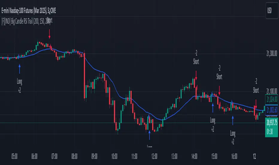
[LTS] Marubozu Candle StrategyOVERVIEW
The Marubozu Candle Strategy identifies and trades wickless candles (Marubozu patterns) with dynamic take-profit and stop-loss levels based on market volatility. This indicator combines traditional Japanese candlestick pattern recognition with modern volatility-adjusted risk management and includes a comprehensive performance tracking dashboard.
A Marubozu candle is a powerful continuation pattern characterized by the complete absence of wicks on one side, indicating strong directional momentum. This strategy specifically detects:
- Bullish Marubozu: Close > Open AND Low = Open (no lower wick)
- Bearish Marubozu: Close < Open AND High = Open (no upper wick)
When price returns to test these levels, the indicator generates trading signals with predefined risk-reward parameters.
CORE METHODOLOGY
Detection Logic:
The script scans each bar for Marubozu formations using precise price comparisons. When a wickless candle appears, a horizontal line extends from the opening price, marking it as a potential support (bullish) or resistance (bearish) level. These levels remain active until price touches them or until the maximum line limit is reached.
EMA Filter (Optional):
An exponential moving average filter enhances signal quality by requiring proper trend alignment. For bullish signals, price must be above the EMA when touching the level. For bearish signals, price must be below the EMA. This filter reduces counter-trend trades and improves win rates in trending markets. Users can disable this filter for range-bound conditions.
Dynamic Risk Management:
The strategy employs ATR-based (Average True Range) position sizing rather than fixed point values. This approach adapts to market volatility automatically:
- In low volatility: Tighter stops and targets
- In high volatility: Wider stops and targets proportional to market movement
Default settings use a 2:1 reward-to-risk ratio (1x ATR for take-profit, 0.5x ATR for stop-loss), but users can adjust these multipliers to match their trading style.
HOW IT WORKS
Step 1 - Pattern Detection:
On each bar, the indicator evaluates whether the candle qualifies as a Marubozu by comparing the high, low, open, and close prices. When detected, the opening price becomes the key level.
Step 2 - Level Management:
Horizontal lines extend from each Marubozu's opening price. The indicator maintains two separate arrays: one for unbroken levels (actively extending) and one for broken levels (historical reference). Users can configure how many of each type to display, preventing chart clutter while maintaining relevant context.
Step 3 - Signal Generation:
When price returns to touch a Marubozu level, the indicator evaluates the EMA filter condition. If the filter passes (or is disabled), the script draws TP/SL boxes showing the expected profit and loss zones based on current ATR values.
Step 4 - Trade Tracking:
Each valid signal enters the tracking system, which monitors subsequent price action to determine outcomes. The script identifies whether the take-profit or stop-loss was hit first (discarding trades where both trigger on the same candle to avoid ambiguous results).
PERFORMANCE DASHBOARD
The integrated dashboard provides real-time strategy analytics to automatically convert results to dollar values for any instrument:
Tracked Metrics:
- Total Trades: Complete count of closed positions
- Wins/Losses: Individual counts with color coding
- Win Rate: Success percentage with dynamic color (green >= 50%, red < 50%)
- Total P&L: Cumulative profit/loss in dollars
- Avg Win: Mean dollar amount per winning trade
- Avg Loss: Mean dollar amount per losing trade
NOTE: The dollar values shown in the dashboard are for trading only a single share/contract/etc. You will need to manually multiply those numbers by the amount of shares/contracts you are trading to get a true value.
The dollar conversion works automatically across all markets:
- Futures contracts (ES, NQ, CL, etc.) use their contract specifications
- Forex pairs use standard lot calculations
- Stocks and crypto use their respective point values
This eliminates manual calculation and provides immediate performance feedback in meaningful currency terms.
CUSTOMIZATION OPTIONS
ATR Settings:
- ATR Period: Lookback length for volatility calculation (default: 14)
- TP Multiplier: Take-profit distance as multiple of ATR (default: 3.0)
- SL Multiplier: Stop-loss distance as multiple of ATR (default: 1.5)
EMA Settings:
- EMA Length: Period for trend filter calculation (default: 9)
- Use EMA Filter: Toggle trend confirmation requirement (default: enabled)
Visual Settings:
- Bullish Color: Color for long signals and wins (default: green)
- Bearish Color: Color for short signals and losses (default: red)
- EMA Color: Color for trend filter line (default: orange)
- Line Width: Thickness of Marubozu level lines (1-5, default: 2)
- EMA Width: Thickness of EMA line (1-5, default: 2)
Line Management:
- Max Unbroken Lines: Limit for active extending lines (default: 10)
- Max Broken Lines: Limit for historical touched lines (default: 5)
Dashboard Settings:
- Show Dashboard: Toggle performance display on/off
- Dashboard Position: Corner placement (4 options)
- Dashboard Size: Text size selection (Tiny/Small/Normal/Large)
HOW TO USE
1. Add the indicator to your chart
2. Adjust ATR multipliers based on your risk tolerance (higher values = more conservative)
3. Configure the EMA filter based on market conditions (enable for trending, disable for ranging)
4. Set line limits to match your visual preference and chart timeframe
5. Monitor the dashboard to track strategy performance in real-time
6. Use the TP/SL boxes as reference levels for manual trades or automation
Best Practices:
- Enable EMA filter in strongly trending markets
- Disable EMA filter if you want more trade signals but at lower quality
- Increase ATR multipliers in highly volatile markets
- Decrease ATR multipliers for tighter, more frequent trades
- Review avg win/loss ratio to ensure positive expectancy
UNIQUE FEATURES
Unlike basic Marubozu detectors, this strategy provides:
1. Automatic level tracking with memory management
2. Volatility-adjusted risk parameters instead of fixed values
3. Optional trend confirmation via EMA filter
4. Real-time performance analytics with automatic dollar conversion
5. Separate tracking of wins/losses with individual averages
6. Configurable visual display to prevent chart clutter
7. Complete transparency with all logic visible in open-source code

Supertrend TP SL (PRO)2. Main Components:
Supertrend Indicator:
Theoretical basis: The Supertrend indicator is based on two main concepts: Average True Range (ATR) and Factor. ATR measures the extent of price fluctuations in a given period of time, while Factor determines the sensitivity of the indicator to price changes.
Mechanism of operation: The indicator calculates two possible lines: one line representing the potential support level and another line representing the potential resistance level. The selection of the appropriate line depends on the current price direction. When the price is above the line, the indicator is considered to be in an uptrend, and vice versa.
Customizable inputs:
atrPeriod: Allows the trader to specify the time period for calculating the ATR. Shorter periods make the indicator more sensitive to price changes, while longer periods reduce its sensitivity.
factor: Allows the adjustment of the factor. Higher values make the indicator less likely to give false signals, but they may also delay entry signals.
Risk Management:
Take Profit and Stop Loss Orders:
TPPoints: Specifies the distance between the entry price and the take profit level. This distance is expressed in points, and is converted to an actual price value using syminfo.mintick (the smallest possible price movement of the traded asset).
SLPoints: Specifies the distance between the entry price and the stop loss level.
Importance: These orders allow the trader to specify the maximum loss he is willing to take and the profit target he is aiming to achieve, which helps in effective risk management.
Activate/Disable Trades:
isLongEnabled: Allows buy trades to be enabled or disabled, which allows the trader to trade in one direction only (for example, only trade in the uptrend during a bull market).
isShortEnabled: Allows sell trades to be enabled or disabled.
isTakeProfitEnabled: Allows take profit orders to be enabled or disabled. The trader may wish to disable them if he prefers to manage his trades manually.
isStopLossEnabled: Allows you to enable or disable stop loss orders. Although disabling them may seem tempting in some cases, it is a very risky move.
Visual Customization:
Line Style and Width:
lineStyle: Allows the trader to choose the style of lines used to draw TP and SL levels (Solid, Dashed, Dotted).
lineWidth: Sets the thickness of the lines.
Label Size:
labelSize: Allows you to set the size of the labels that display TP and SL levels (Small, Normal, Large).
Colors:
bullColor, bearColor, tpColor, slColor: Allows the trader to customize the colors of the different elements on the chart, making visual analysis easier.
3. Strategy Logic:
Determining Entry Signals: The strategy relies on the Supertrend indicator to determine entry signals. When the Supertrend trend changes from bearish to bullish, a buy trade is triggered (if isLongEnabled is enabled). When the trend changes from bullish to bearish, a sell trade is triggered (if isShortEnabled is enabled).
Order Execution: Once the entry signal is triggered, the strategy automatically places buy or sell orders.
Trade Management: After opening a trade, the strategy monitors the price and automatically triggers Take Profit and Stop Loss orders if the price reaches the specified levels.
Visualization: The strategy displays useful information on the chart, such as TP and SL lines, entry and exit signals, which helps the trader understand the strategy’s behavior and evaluate its performance.
4. Advanced Tips:
Optimizing Settings: The strategy’s performance can be improved by adjusting different input values. For example, the trader can experiment with different values for atrPeriod and factor to improve the accuracy of Supertrend signals.
Combining Indicators: This strategy can be combined with other indicators to improve the accuracy of entry signals. For example, the Relative Strength Index (RSI) can be used to confirm Supertrend signals.
Time Analysis: The strategy’s performance can be analyzed over different time periods to evaluate its effectiveness in various market conditions.
Strategy Testing: Before using the strategy in real trading, it should be tested on historical data (Backtesting) to evaluate its performance and determine the optimal settings.
5. Associated Risks:
False Signals: The Supertrend indicator may sometimes give false signals, especially in volatile markets.
Losses: Even with the use of stop loss orders, the trader may be exposed to significant losses.
Over-optimization: Over-optimization of settings on historical data may lead to misleading results. The trader should be careful about generalizing the results to future data.
Over-reliance on automation: The automated strategy should not be relied upon completely. The trader should monitor the trades and make appropriate decisions when necessary.
6. Disclaimer:
I am not a licensed financial advisor. This strategy is provided for educational and illustrative purposes only and should not be considered as investment advice. Trading in financial markets involves significant risks and you may lose your invested capital. Before making any investment decisions, consult a qualified financial advisor and conduct your own research. You alone are responsible for your trading decisions and their results. By using this strategy, you acknowledge and agree that I am not responsible for any losses or damages you may incur.
2. المكونات الرئيسية:
مؤشر Supertrend:
الأساس النظري: يعتمد مؤشر Supertrend على مفهومين رئيسيين هما: متوسط المدى الحقيقي (Average True Range - ATR) ومعامل الضرب (Factor). ATR يقيس مدى تقلبات الأسعار في فترة زمنية محددة، بينما Factor يحدد مدى حساسية المؤشر لتغيرات الأسعار.
آلية العمل: يقوم المؤشر بحساب خطين محتملين: خط يمثل مستوى الدعم المحتمل وخط آخر يمثل مستوى المقاومة المحتمل. يعتمد اختيار الخط المناسب على اتجاه السعر الحالي. عندما يكون السعر أعلى من الخط، يعتبر المؤشر في اتجاه صاعد، والعكس صحيح.
المدخلات القابلة للتخصيص:
atrPeriod: يتيح للمتداول تحديد الفترة الزمنية لحساب ATR. الفترات الأقصر تجعل المؤشر أكثر حساسية لتغيرات الأسعار، بينما الفترات الأطول تقلل من حساسيته.
factor: يسمح بتعديل معامل الضرب. القيم الأعلى تجعل المؤشر أقل عرضة لإعطاء إشارات خاطئة، ولكنها قد تؤخر أيضًا إشارات الدخول.
إدارة المخاطر:
أوامر جني الأرباح وإيقاف الخسارة:
TPPoints: يحدد المسافة بين سعر الدخول ومستوى جني الأرباح. يتم التعبير عن هذه المسافة بالنقاط (Points)، ويتم تحويلها إلى قيمة سعرية فعلية باستخدام syminfo.mintick (أصغر حركة سعرية ممكنة للأصل المتداول).
SLPoints: يحدد المسافة بين سعر الدخول ومستوى إيقاف الخسارة.
الأهمية: تتيح هذه الأوامر للمتداول تحديد الحد الأقصى للخسارة التي يرغب في تحملها والهدف الربحي الذي يسعى لتحقيقه، مما يساعد على إدارة المخاطر بشكل فعال.
تفعيل/تعطيل الصفقات:
isLongEnabled: يسمح بتفعيل أو تعطيل صفقات الشراء، مما يمكن المتداول من التداول في اتجاه واحد فقط (على سبيل المثال، التداول فقط في الاتجاه الصاعد خلال سوق صاعدة).
isShortEnabled: يسمح بتفعيل أو تعطيل صفقات البيع.
isTakeProfitEnabled: يسمح بتفعيل أو تعطيل أوامر جني الأرباح. قد يرغب المتداول في تعطيلها إذا كان يفضل إدارة صفقاته يدويًا.
isStopLossEnabled: يسمح بتفعيل أو تعطيل أوامر إيقاف الخسارة. على الرغم من أن تعطيلها قد يبدو مغريًا في بعض الحالات، إلا أنه يعتبر خطوة محفوفة بالمخاطر للغاية.
التخصيص المرئي:
نمط وعرض الخطوط:
lineStyle: يتيح للمتداول اختيار نمط الخطوط المستخدمة لرسم مستويات TP و SL (Solid, Dashed, Dotted).
lineWidth: يحدد سمك الخطوط.
حجم الملصقات:
labelSize: يسمح بتحديد حجم الملصقات التي تعرض مستويات TP و SL (Small, Normal, Large).
الألوان:
bullColor, bearColor, tpColor, slColor: تتيح للمتداول تخصيص ألوان العناصر المختلفة على الرسم البياني، مما يسهل عملية التحليل البصري.
3. منطق عمل الاستراتيجية:
تحديد إشارات الدخول: تعتمد الاستراتيجية على مؤشر Supertrend لتحديد إشارات الدخول. عندما يتغير اتجاه Supertrend من هابط إلى صاعد، يتم تفعيل صفقة شراء (إذا كانت isLongEnabled مفعلة). وعندما يتغير الاتجاه من صاعد إلى هابط، يتم تفعيل صفقة بيع (إذا كانت isShortEnabled مفعلة).
تنفيذ الأوامر: بمجرد تفعيل إشارة الدخول، تقوم الاستراتيجية بوضع أوامر الشراء أو البيع تلقائيًا.
إدارة الصفقات: بعد فتح الصفقة، تقوم الاستراتيجية بمراقبة السعر وتفعيل أوامر جني الأرباح وإيقاف الخسارة تلقائيًا في حالة وصول السعر إلى المستويات المحددة.
التمثيل المرئي: تعرض الاستراتيجية معلومات مفيدة على الرسم البياني، مثل خطوط TP و SL وإشارات الدخول والخروج، مما يساعد المتداول على فهم سلوك الاستراتيجية وتقييم أدائها.
4. نصائح متقدمة:
تحسين الإعدادات: يمكن تحسين أداء الاستراتيجية من خلال تعديل قيم المدخلات المختلفة. على سبيل المثال، يمكن للمتداول تجربة قيم مختلفة لـ atrPeriod و factor لتحسين دقة إشارات Supertrend.
الجمع بين المؤشرات: يمكن دمج هذه الاستراتيجية مع مؤشرات أخرى لتحسين دقة إشارات الدخول. على سبيل المثال، يمكن استخدام مؤشر القوة النسبية (RSI) لتأكيد إشارات Supertrend.
التحليل الزمني: يمكن تحليل أداء الاستراتيجية على مدى فترات زمنية مختلفة لتقييم مدى فعاليتها في ظروف السوق المتنوعة.
اختبار الاستراتيجية: قبل استخدام الاستراتيجية في التداول الحقيقي، يجب اختبارها على بيانات تاريخية (Backtesting) لتقييم أدائها وتحديد الإعدادات المثلى.
5. المخاطر المرتبطة:
الإشارات الخاطئة: قد يعطي مؤشر Supertrend إشارات خاطئة في بعض الأحيان، خاصة في الأسواق المتقلبة.
الخسائر: حتى مع استخدام أوامر إيقاف الخسارة، قد يتعرض المتداول لخسائر كبيرة.
التحسين المفرط: قد يؤدي التحسين المفرط للإعدادات على بيانات تاريخية إلى نتائج مضللة. يجب أن يكون المتداول حذرًا بشأن تعميم النتائج على البيانات المستقبلية.
الاعتماد الزائد على الأتمتة: يجب عدم الاعتماد بشكل كامل على الاستراتيجية الآلية. يجب على المتداول مراقبة الصفقات واتخاذ القرارات المناسبة عند الضرورة.
6. إخلاء المسؤولية:
أنا لست مستشارًا ماليًا مرخصًا. هذه الاستراتيجية مقدمة لأغراض تعليمية وتوضيحية فقط، ولا ينبغي اعتبارها نصيحة استثمارية. التداول في الأسواق المالية ينطوي على مخاطر كبيرة، وقد تخسر رأس المال المستثمر. قبل اتخاذ أي قرارات استثمارية، استشر مستشارًا ماليًا مؤهلاً وقم بإجراء بحثك الخاص. أنت وحدك المسؤول عن قراراتك التجارية ونتائجها. باستخدام هذه الاستراتيجية، فإنك تقر وتوافق على أنني لست مسؤولاً عن أي خسائر أو أضرار قد تتكبدها.

Long-Only Opening Range Breakout (ORB) with Pivot PointsIntraday Trading Strategy: Long-Only Opening Range Breakout (ORB) with Pivot Points
Background:
Opening Range Breakout (ORB) is a popular long-only trading strategy that capitalizes on the early morning volatility in financial markets. It's based on the idea that the initial price movements during the first few minutes or hours of the trading day can set the tone for the rest of the session. The strategy involves identifying a price range within which the asset trades during the opening period and then taking long positions when the price breaks out to the upside of this range.
Pivot Points are a widely used technical indicator in trading. They represent potential support and resistance levels based on the previous day's price action. Pivot points are calculated using the previous day's high, low, and close prices and can help traders identify key price levels for making trading decisions.
How to Use the Script:
Initialization: This script is written in Pine Script, a domain-specific language for trading strategies on the TradingView platform. To use this script, you need to have access to TradingView.
Apply the Script: You can do this by adding it to your favorites, then selecting the script in the indicators list under favorites or by searching for it by name under community scripts.
Customize Settings: The script allows you to customize various settings through the TradingView interface. These settings include:
Opening Session: You can set the time frame for the opening session.
Max Trades per Day: Specify the maximum number of long trades allowed per trading day.
Initial Stop Loss Type: Choose between using a percentage-based stop loss or the previous candles low for stop loss calculations.
Stop Loss Percentage: If you select the percentage-based stop loss, specify the percentage of the entry price for the stop loss.
Backtesting Start and End Time: Set the time frame for backtesting the strategy.
Strategy Signals:
The script will display pivot points in blue (R1, R2, R3, R4, R5) and half-pivot points in gray (R0.5, R1.5, R2.5, R3.5, R4.5) on your chart.
The green line represents the opening range.
The script generates long (buy) signals based on specific conditions:
---The open price is below the opening range high (h).
---The current high price is above the opening range high.
---Pivot point R1 is above the opening range high.
---It's a long-only strategy designed to capture upside breakouts.
---It also respects the maximum number of long trades per day.
The script manages long positions, calculates stop losses, and adjusts long positions according to the defined rules.
Trailing Stop Mechanism
The script incorporates a dynamic trailing stop mechanism designed to protect and maximize profits for long positions. Here's how it works:
1. Initialization:
The script allows you to choose between two types of initial stop loss:
---Percentage-based: This option sets the initial stop loss as a percentage of the entry price.
---Previous day's low: This option sets the initial stop loss at the previous day's low.
2. Setting the Initial Stop Loss (`sl_long0`):
The initial stop loss (`sl_long0`) is calculated based on the chosen method:
---If "Percentage" is selected, it calculates the stop loss as a percentage of the entry price.
---If "Previous Low" is selected, it sets the stop loss at the previous day's low.
3. Dynamic Trailing Stop (`trail_long`):
The script then monitors price movements and uses a dynamic trailing stop mechanism (`trail_long`) to adjust the stop loss level for long positions.
If the current high price rises above certain pivot point levels, the trailing stop is adjusted upwards to lock in profits.
The trailing stop levels are calculated based on pivot points (`r1`, `r2`, `r3`, etc.) and half-pivot points (`r0.5`, `r1.5`, `r2.5`, etc.).
The script checks if the high price surpasses these levels and, if so, updates the trailing stop accordingly.
This dynamic trailing stop allows traders to secure profits while giving the position room to potentially capture additional gains.
4. Final Stop Loss (`sl_long`):
The script calculates the final stop loss level (`sl_long`) based on the following logic:
---If no position is open (`pos == 0`), the stop loss is set to zero, indicating there is no active stop loss.
---If a position is open (`pos == 1`), the script calculates the maximum of the initial stop loss (`sl_long0`) and the dynamic trailing stop (`trail_long`).
---This ensures that the stop loss is always set to the more conservative of the two values to protect profits.
5. Plotting the Stop Loss:
The script plots the stop loss level on the chart using the `plot` function.
It will only display the stop loss level if there is an open position (`pos == 1`) and it's not a new trading day (`not newday`).
The stop loss level is shown in red on the chart.
By combining an initial stop loss with a dynamic trailing stop based on pivot points and half-pivot points, the script aims to provide a comprehensive risk management mechanism for long positions. This allows traders to lock in profits as the price moves in their favor while maintaining a safeguard against adverse price movements.
End of Day (EOD) Exit:
The script includes an "End of Day" (EOD) exit mechanism to automatically close any open positions at the end of the trading day. This feature is designed to manage and control positions when the trading day comes to a close. Here's how it works:
1. Initialization:
At the beginning of each trading day, the script identifies a new trading day using the `is_newbar('D')` condition.
When a new trading day begins, the `newday` variable becomes `true`, indicating the start of a new trading session.
2. Plotting the "End of Day" Signal:
The script includes a plot on the chart to visually represent the "End of Day" signal. This is done using the `plot` function.
The plot is labeled "DayEnd" and is displayed as a comment on the chart. It signifies the EOD point.
3. EOD Exit Condition:
When the script detects that a new trading day has started (`newday == true`), it triggers the EOD exit condition.
At this point, the script proceeds to close all open positions that may have been active during the trading day.
4. Closing Open Positions:
The `strategy.close_all` function is used to close all open positions when the EOD exit condition is met.
This function ensures that any remaining long positions are exited, regardless of their current profit or loss.
The function also includes an `alert_message`, which can be customized to send an alert or notification when positions are closed at EOD.
Purpose of EOD Exit
The "End of Day" exit mechanism serves several essential purposes in the trading strategy:
Risk Management: It helps manage risk by ensuring that positions are not left open overnight when markets can experience increased volatility.
Capital Preservation: Closing positions at EOD can help preserve trading capital by avoiding potential adverse overnight price movements.
Rule-Based Exit: The EOD exit is rule-based and automatic, ensuring that it is consistently applied without emotions or manual intervention.
Scalability: It allows the strategy to be applied to various markets and timeframes where EOD exits may be appropriate.
By incorporating an EOD exit mechanism, the script provides a comprehensive approach to managing positions, taking profits, and minimizing risk as each trading day concludes. This can be especially important in volatile markets like cryptocurrencies, where overnight price swings can be significant.
Backtesting: The script includes a backtesting feature that allows you to test the strategy's performance over historical data. Set the start and end times for backtesting to see how the long-only strategy would have performed in the past.
Trade Execution: If you choose to use this script for live trading, make sure you understand the risks involved. It's essential to set up proper risk management, including position sizing and stop loss orders.
Monitoring: Monitor the long-only strategy's performance over time and be prepared to make adjustments as market conditions change.
Disclaimer: Trading carries a risk of capital loss. This script is provided for educational purposes and as a starting point for your own long-only strategy development. Always do your own research and consider seeking advice from a qualified financial professional before making trading decisions.

Stochastic Hash Strat [Hash Capital Research]# Stochastic Hash Strategy by Hash Capital Research
## 🎯 What Is This Strategy?
The **Stochastic Slow Strategy** is a momentum-based trading system that identifies oversold and overbought market conditions to capture mean-reversion opportunities. Think of it as a "buy low, sell high" approach with smart mathematical filters that remove emotion from your trading decisions.
Unlike fast-moving indicators that generate excessive noise, this strategy uses **smoothed stochastic oscillators** to identify only the highest-probability setups when momentum truly shifts.
---
## 💡 Why This Strategy Works
Most traders fail because they:
- **Chase prices** after big moves (buying high, selling low)
- **Overtrade** in choppy, directionless markets
- **Exit too early** or hold losses too long
This strategy solves all three problems:
1. **Entry Discipline**: Only trades when the stochastic oscillator crosses in extreme zones (oversold for longs, overbought for shorts)
2. **Cooldown Filter**: Prevents revenge trading by forcing a waiting period after each trade
3. **Fixed Risk/Reward**: Pre-defined stop-loss and take-profit levels ensure consistent risk management
**The Math Behind It**: The stochastic oscillator measures where the current price sits relative to its recent high-low range. When it's below 25, the market is oversold (time to buy). When above 70, it's overbought (time to sell). The crossover with its moving average confirms momentum is shifting.
---
## 📊 Best Markets & Timeframes
### ⭐ OPTIMAL PERFORMANCE:
**Crude Oil (WTI) - 12H Timeframe**
- **Why it works**: Oil markets have predictable volatility patterns and respect technical levels
**AAVE/USD - 4H to 12H Timeframe**
- **Why it works**: DeFi tokens exhibit strong momentum cycles with clear extremes
### ✅ Also Works Well On:
- **BTC/USD** (12H, Daily) - Lower frequency but high win rate
- **ETH/USD** (8H, 12H) - Balanced volatility and liquidity
- **Gold (XAU/USD)** (Daily) - Classic mean-reversion asset
- **EUR/USD** (4H, 8H) - Lower volatility, requires patience
### ❌ Avoid Using On:
- Timeframes below 4H (too much noise)
- Low-liquidity altcoins (wide spreads kill performance)
- Strongly trending markets without pullbacks (Bitcoin in 2021)
- News-driven instruments during major events
---
## 🎛️ Understanding The Settings
### Core Stochastic Parameters
**Stochastic Length (Default: 16)**
- Controls the lookback period for price comparison
- Lower = faster reactions, more signals (10-14 for volatile markets)
- Higher = smoother signals, fewer trades (16-21 for stable markets)
- **Pro tip**: Use 10 for crypto 4H, 16 for commodities 12H
**Overbought Level (Default: 70)**
- Threshold for short entries
- Lower values (65-70) = more trades, earlier entries
- Higher values (75-80) = fewer but higher-conviction trades
- **Sweet spot**: 70 works for most assets
**Oversold Level (Default: 25)**
- Threshold for long entries
- Higher values (25-30) = more trades, earlier entries
- Lower values (15-20) = fewer but stronger bounce setups
- **Sweet spot**: 20-25 depending on market conditions
**Smooth K & Smooth D (Default: 7 & 3)**
- Additional smoothing to filter out whipsaws
- K=7 makes the indicator slower and more reliable
- D=3 is the signal line that confirms the trend
- **Don't change these unless you know what you're doing**
---
### Risk Management
**Stop Loss % (Default: 2.2%)**
- Automatically exits losing trades
- Should be 1.5x to 2x your average market volatility
- Too tight = death by a thousand cuts
- Too wide = uncontrolled losses
- **Calibration**: Check ATR indicator and set SL slightly above it
**Take Profit % (Default: 7%)**
- Automatically exits winning trades
- Should be 2.5x to 3x your stop loss (reward-to-risk ratio)
- This default gives 7% / 2.2% = 3.18:1 R:R
- **The golden rule**: Never have R:R below 2:1
---
### Trade Filters
**Bar Cooldown Filter (Default: ON, 3 bars)**
- **What it does**: Forces you to wait X bars after closing a trade before entering a new one
- **Why it matters**: Prevents emotional revenge trading and overtrading in choppy markets
- **Settings guide**:
- 3 bars = Standard (good for most cases)
- 5-7 bars = Conservative (oil, slow-moving assets)
- 1-2 bars = Aggressive (only for experienced traders)
**Exit on Opposite Extreme (Default: ON)**
- Closes your long when stochastic hits overbought (and vice versa)
- Acts as an early profit-taking mechanism
- **Leave this ON** unless you're testing other exit strategies
**Divergence Filter (Default: OFF)**
- Looks for price/momentum divergences for additional confirmation
- **When to enable**: Trending markets where you want fewer but higher-quality trades
- **Keep OFF for**: Mean-reverting markets (oil, forex, most of the time)
---
## 🚀 Quick Start Guide
### Step 1: Set Up in TradingView
1. Open TradingView and navigate to your chart
2. Click "Pine Editor" at the bottom
3. Copy and paste the strategy code
4. Click "Add to Chart"
5. The strategy will appear in a separate pane below your price chart
### Step 2: Choose Your Market
**If you're trading Crude Oil:**
- Timeframe: 12H
- Keep all default settings
- Watch for signals during London/NY overlap (8am-11am EST)
**If you're trading AAVE or crypto:**
- Timeframe: 4H or 12H
- Consider these adjustments:
- Stochastic Length: 10-14 (faster)
- Oversold: 20 (more aggressive)
- Take Profit: 8-10% (higher targets)
### Step 3: Wait for Your First Signal
**LONG Entry** (Green circle appears):
- Stochastic crosses up below oversold level (25)
- Price likely near recent lows
- System places limit order at take profit and stop loss
**SHORT Entry** (Red circle appears):
- Stochastic crosses down above overbought level (70)
- Price likely near recent highs
- System places limit order at take profit and stop loss
**EXIT** (Orange circle):
- Position closes either at stop, target, or opposite extreme
- Cooldown period begins
### Step 4: Let It Run
The biggest mistake? **Interfering with the system.**
- Don't close trades early because you're scared
- Don't skip signals because you "have a feeling"
- Don't increase position size after a big win
- Don't revenge trade after a loss
**Follow the system or don't use it at all.**
---
### Important Risks:
1. **Drawdown Pain**: You WILL experience losing streaks of 5-7 trades. This is mathematically normal.
2. **Whipsaw Markets**: Choppy, range-bound conditions can trigger multiple small losses.
3. **Gap Risk**: Overnight gaps can cause your actual fill to be worse than the stop loss.
4. **Slippage**: Real execution prices differ from backtested prices (factor in 0.1-0.2% slippage).
---
## 🔧 Optimization Guide
### When to Adjust Settings:
**Market Volatility Increased?**
- Widen stop loss by 0.5-1%
- Increase take profit proportionally
- Consider increasing cooldown to 5-7 bars
**Getting Too Few Signals?**
- Decrease stochastic length to 10-12
- Increase oversold to 30, decrease overbought to 65
- Reduce cooldown to 2 bars
**Getting Too Many Losses?**
- Increase stochastic length to 18-21 (slower, smoother)
- Enable divergence filter
- Increase cooldown to 5+ bars
- Verify you're on the right timeframe
### A/B Testing Method:
1. **Run default settings for 50 trades** on your chosen market
2. Document: Win rate, profit factor, max drawdown, emotional tolerance
3. **Change ONE variable** (e.g., oversold from 25 to 20)
4. Run another 50 trades
5. Compare results
6. Keep the better version
**Never change multiple settings at once** or you won't know what worked.
---
## 📚 Educational Resources
### Key Concepts to Learn:
**Stochastic Oscillator**
- Developed by George Lane in the 1950s
- Measures momentum by comparing closing price to price range
- Formula: %K = (Close - Low) / (High - Low) × 100
- Similar to RSI but more sensitive to price movements
**Mean Reversion vs. Trend Following**
- This is a **mean reversion** strategy (price returns to average)
- Works best in ranging markets with defined support/resistance
- Fails in strong trending markets (2017 Bitcoin, 2020 Tech stocks)
- Complement with trend filters for better results
**Risk:Reward Ratio**
- The cornerstone of profitable trading
- Winning 40% of trades with 3:1 R:R = profitable
- Winning 60% of trades with 1:1 R:R = breakeven (after fees)
- **This strategy aims for 45% win rate with 2.5-3:1 R:R**
### Recommended Reading:
- *"Trading Systems and Methods"* by Perry Kaufman (Chapter on Oscillators)
- *"Mean Reversion Trading Systems"* by Howard Bandy
- *"The New Trading for a Living"* by Dr. Alexander Elder
---
## 🛠️ Troubleshooting
### "I'm not seeing any signals!"
**Check:**
- Is your timeframe 4H or higher?
- Is the stochastic actually reaching extreme levels (check if your asset is stuck in middle range)?
- Is cooldown still active from a previous trade?
- Are you on a low-liquidity pair?
**Solution**: Switch to a more volatile asset or lower the overbought/oversold thresholds.
---
### "The strategy keeps losing money!"
**Check:**
- What's your win rate? (Below 35% is concerning)
- What's your profit factor? (Below 0.8 means serious issues)
- Are you trading during major news events?
- Is the market in a strong trend?
**Solution**:
1. Verify you're using recommended markets/timeframes
2. Increase cooldown period to avoid choppy markets
3. Reduce position size to 5% while you diagnose
4. Consider switching to daily timeframe for less noise
---
### "My stop losses keep getting hit!"
**Check:**
- Is your stop loss tighter than the average ATR?
- Are you trading during high-volatility sessions?
- Is slippage eating into your buffer?
**Solution**:
1. Calculate the 14-period ATR
2. Set stop loss to 1.5x the ATR value
3. Avoid trading right after market open or major news
4. Factor in 0.2% slippage for crypto, 0.1% for oil
---
## 💪 Pro Tips from the Trenches
### Psychological Discipline
**The Three Deadly Sins:**
1. **Skipping signals** - "This one doesn't feel right"
2. **Early exits** - "I'll just take profit here to be safe"
3. **Revenge trading** - "I need to make back that loss NOW"
**The Solution:** Treat your strategy like a business system. Would McDonald's skip making fries because the cashier "doesn't feel like it today"? No. Systems work because of consistency.
---
### Position Management
**Scaling In/Out** (Advanced)
- Enter 50% position at signal
- Add 50% if stochastic reaches 10 (oversold) or 90 (overbought)
- Exit 50% at 1.5x take profit, let the rest run
**This is NOT for beginners.** Master the basic system first.
---
### Market Awareness
**Oil Traders:**
- OPEC meetings = volatility spikes (avoid or widen stops)
- US inventory reports (Wed 10:30am EST) = avoid trading 2 hours before/after
- Summer driving season = different patterns than winter
**Crypto Traders:**
- Monday-Tuesday = typically lower volatility (fewer signals)
- Thursday-Sunday = higher volatility (more signals)
- Avoid trading during exchange maintenance windows
---
## ⚖️ Legal Disclaimer
This trading strategy is provided for **educational purposes only**.
- Past performance does not guarantee future results
- Trading involves substantial risk of loss
- Only trade with capital you can afford to lose
- No one associated with this strategy is a licensed financial advisor
- You are solely responsible for your trading decisions
**By using this strategy, you acknowledge that you understand and accept these risks.**
---
## 🙏 Acknowledgments
Strategy development inspired by:
- George Lane's original Stochastic Oscillator work
- Modern quantitative trading research
- Community feedback from hundreds of backtests
Built with ❤️ for retail traders who want systematic, disciplined approaches to the markets.
---
**Good luck, stay disciplined, and trade the system, not your emotions.**
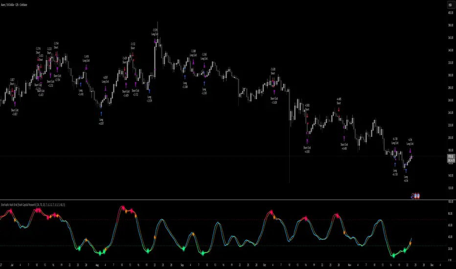
Hash Momentum Strategy# Hash Momentum Strategy
## 📊 Overview
The **Hash Momentum Strategy** is a professional-grade momentum trading system designed to capture strong directional price movements with precision timing and intelligent risk management. Unlike traditional EMA crossover strategies, this system uses momentum acceleration as its primary signal, resulting in earlier entries and better risk-to-reward ratios.
---
## ⚡ What Makes This Strategy Unique
### 1. Momentum-Based Entry System
Most strategies rely on lagging indicators like moving average crossovers. This strategy captures momentum *acceleration* - entering when price movement is gaining strength, not after the move has already happened.
### 2. Programmable Risk-to-Reward
Set your exact R:R ratio (1:2, 1:2.5, 1:3, etc.) and the strategy automatically calculates stop loss and take profit levels. No more guessing or manual calculations.
### 3. Smart Partial Profit Taking
Lock in profits at multiple stages:
- **First TP**: Take 50% off at 2R
- **Second TP**: Take 40% off at 2.5R
- **Final TP**: Let 10% ride to maximum target
This approach locks in gains while letting winners run.
### 4. Dynamic Momentum Threshold
Uses ATR (Average True Range) multiplied by your threshold setting to adapt to market volatility. Volatile markets = higher threshold. Quiet markets = lower threshold.
### 5. Trade Cooldown System
Prevents overtrading and revenge trading by enforcing a cooldown period between trades. Configurable from 1-24 bars.
### 6. Optional Session & Weekend Filters
Filter trades by Tokyo, London, and New York sessions. Optional weekend-off toggle to avoid low-liquidity periods.
---
## 🎯 How It Works
### Signal Generation
**STEP 1: Calculate Momentum**
- Momentum = Current Price - Price
- Check if Momentum > ATR × Threshold Multiplier
- Momentum must be accelerating (positive change in momentum)
**STEP 2: Confirm with EMA Trend Filter**
- Long: Price must be above EMA
- Short: Price must be below EMA
**STEP 3: Check Filters**
- Not in cooldown period
- Valid session (if enabled)
- Not weekend (if enabled)
**STEP 4: ENTRY SIGNAL TRIGGERED**
### Risk Management Example
**Example Long Trade:**
- Entry: $100
- Stop Loss: $97.80 (2.2% risk)
- Risk Amount: $2.20
**Take Profit Levels:**
- TP1: $104.40 (2R = $4.40) → Close 50%
- TP2: $105.50 (2.5R = $5.50) → Close 40%
- Final: $105.50 (2.5R) → Close remaining 10%
---
## ⚙️ Settings Guide
### Core Strategy
**Momentum Length** (Default: 13)
Number of bars for momentum calculation. Higher = stronger but fewer signals.
**Momentum Threshold** (Default: 2.25)
ATR multiplier. Higher = only trade biggest moves.
**Use EMA Trend Filter** (Default: ON)
Only long above EMA, short below EMA.
**EMA Length** (Default: 28)
Period for trend-confirming EMA.
### Filters
**Use Trading Session Filter** (Default: OFF)
Restrict trading to specific sessions.
**Tokyo Session** (Default: OFF)
Trade during Asian hours (00:00-09:00 JST).
**London Session** (Default: OFF)
Trade during European hours (08:00-17:00 GMT).
**New York Session** (Default: OFF)
Trade during US hours (08:00-17:00 EST).
**Weekend Off** (Default: OFF)
Disable trading on Saturdays and Sundays.
### Risk Management
**Stop Loss %** (Default: 2.2)
Fixed percentage stop loss from entry.
**Risk:Reward Ratio** (Default: 2.5)
Your target reward as multiple of risk.
**Use Partial Profit Taking** (Default: ON)
Take profits in stages.
**First TP R:R** (Default: 2.0)
First target as multiple of risk.
**First TP Size %** (Default: 50)
Percentage of position to close at TP1.
**Second TP R:R** (Default: 2.5)
Second target as multiple of risk.
**Second TP Size %** (Default: 40)
Percentage of position to close at TP2.
### Trade Management
**Use Trade Cooldown** (Default: ON)
Prevent overtrading.
**Cooldown Bars** (Default: 6)
Bars to wait after closing a trade.
---
## 🎨 Visual Elements
### Chart Indicators
🟢 **Green Dot** (below bar) = Long entry signal
🔴 **Red Dot** (above bar) = Short entry signal
🔵 **Blue X** (above bar) = Long position closed
🟠 **Orange X** (below bar) = Short position closed
**EMA Line** = Trend direction (green when bullish, red when bearish)
**White Line** = Entry price
**Red Line** = Stop loss level
**Green Lines** = Take profit levels (TP1, TP2, Final)
### Dashboard
When not in real-time mode, a dashboard displays:
- Current position (LONG/SHORT/FLAT)
- Entry price
- Stop loss price
- Take profit price
- R:R ratio
- Current momentum strength
- Total trades
- Win rate
- Net profit %
---
## 📈 Recommended Settings by Timeframe
### 1-Hour Timeframe (Default)
- Momentum Length: 13
- Momentum Threshold: 2.25
- EMA Length: 28
- Stop Loss: 2.2%
- R:R Ratio: 2.5
- Cooldown: 6 bars
### 4-Hour Timeframe
- Momentum Length: 24-36
- Momentum Threshold: 2.5
- EMA Length: 50
- Stop Loss: 3-4%
- R:R Ratio: 2.0-2.5
- Cooldown: 6-8 bars
### 15-Minute Timeframe
- Momentum Length: 8-10
- Momentum Threshold: 2.0
- EMA Length: 20
- Stop Loss: 1.5-2%
- R:R Ratio: 2.0
- Cooldown: 4-6 bars
---
## 🔧 Optimization Tips
### Want More Trades?
- Decrease Momentum Threshold (2.0 instead of 2.25)
- Decrease Momentum Length (10 instead of 13)
- Decrease Cooldown Bars (4 instead of 6)
### Want Higher Quality Trades?
- Increase Momentum Threshold (2.5-3.0)
- Increase Momentum Length (18-24)
- Increase Cooldown Bars (8-10)
### Want Lower Drawdown?
- Increase Cooldown Bars
- Use tighter stop loss
- Enable session filters (trade only high-liquidity sessions)
- Enable Weekend Off
### Want Higher Win Rate?
- Increase R:R Ratio (may reduce total profit)
- Increase Momentum Threshold (fewer but stronger signals)
- Use longer EMA for trend confirmation
---
## 📊 Performance Expectations
Based on typical backtesting results:
- **Win Rate**: 35-45%
- **Profit Factor**: 1.5-2.0
- **Risk:Reward**: 1:2.5 (configurable)
- **Max Drawdown**: 10-20%
- **Trades/Month**: 8-15 (1H timeframe)
**Note:** Win rate may appear low, but with 2.5:1 R:R, you only need ~29% win rate to break even. The strategy aims for quality over quantity.
---
## 🎓 Strategy Logic Explained
### Why Momentum > EMA Crossover?
**EMA Crossover Problems:**
- Signals lag behind price
- Late entries = poor R:R
- Many false signals in ranging markets
**Momentum Advantages:**
- Catches moves as they start accelerating
- Earlier entries = better R:R
- Adapts to volatility via ATR
### Why Partial Profit Taking?
**Without Partial TPs:**
- All-or-nothing approach
- Winners often turn to losers
- High stress watching open positions
**With Partial TPs:**
- Lock in 50% at first target
- Reduce risk to breakeven
- Let remainder ride for bigger gains
- Lower psychological pressure
### Why Trade Cooldown?
**Without Cooldown:**
- Revenge trading after losses
- Overtrading in choppy markets
- Emotional decision-making
**With Cooldown:**
- Forces discipline
- Waits for new setup to develop
- Reduces transaction costs
- Better signal quality
---
## ⚠️ Important Notes
1. **This is a momentum strategy, not an EMA strategy**
The EMA only confirms trend direction. Momentum generates the actual signals.
2. **Backtest thoroughly before live trading**
Past performance ≠ future results. Test on your specific asset and timeframe.
3. **Use proper position sizing**
Risk 1-2% of account per trade maximum. The strategy uses 100% equity by default (adjust in Properties).
4. **Dashboard auto-hides in real-time**
Clean chart for live trading. Visible during backtesting.
5. **Customize for your trading style**
All settings are fully adjustable. No single "best" configuration.
---
## 🚀 Quick Start Guide
1. **Add to Chart**: Apply to your preferred asset and timeframe
2. **Keep Defaults**: Start with default settings
3. **Backtest**: Review historical performance
4. **Paper Trade**: Test with simulated money first
5. **Go Live**: Start small and scale up
---
## 💡 Pro Tips
**Tip 1: Combine Timeframes**
Use higher timeframe (4H) for trend direction, lower timeframe (1H) for entries.
**Tip 2: Avoid News Events**
Major news can cause whipsaws. Consider manual intervention during high-impact events.
**Tip 3: Monitor Momentum Strength**
Dashboard shows momentum in sigma (σ). Values >1.0σ indicate very strong momentum.
**Tip 4: Adjust for Volatility**
In high-volatility markets, increase threshold and stop loss. In quiet markets, decrease them.
**Tip 5: Review Losing Trades**
Check if losses are hitting stop loss or reversing. Adjust stop accordingly.
---
## 📝 Changelog
**v1.0** - Initial Release
- Momentum-based signal generation
- EMA trend filter
- Programmable R:R ratio
- Partial profit taking (3 stages)
- Trade cooldown system
- Session filters (Tokyo/London/New York)
- Weekend off toggle
- Smart dashboard (auto-hides in real-time)
- Clean visual design
---
## 🙏 Credits
Developed by **Hash Capital Research**
If you find this strategy useful, please give it a like and share with others!
---
## ⚖️ Disclaimer
This strategy is for educational purposes only. Trading involves substantial risk of loss and is not suitable for all investors. Past performance is not indicative of future results. Always do your own research and consult with a qualified financial advisor before trading.
---
## 📬 Feedback
Have suggestions or found a bug? Leave a comment below! I'm continuously improving this strategy based on community feedback.
---
**Happy Trading! 🚀📈**
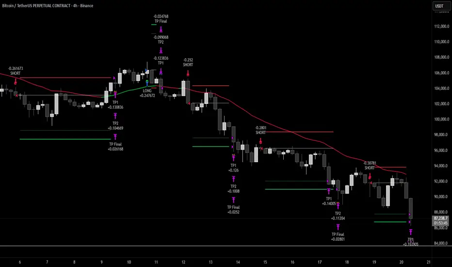
[Parth🇮🇳] Wall Street US30 Pro - Prop Firm Edition....Yo perfect! Here's the COMPLETE strategy in simple words:
***
## WALL STREET US30 TRADING STRATEGY - SIMPLE VERSION
### WHAT YOU'RE TRADING:
US30 (Dow Jones Index) on 1-hour chart using a professional indicator with smart money concepts.
---
### WHEN TO TRADE:
**6:30 PM - 10:00 PM IST every day** (London-NY overlap = highest volume)
***
### THE INDICATOR SHOWS YOU:
A table in top-right corner with 5 things:
1. **Signal Strength** - How confident (need 70%+)
2. **RSI** - Momentum (need OK status)
3. **MACD** - Trend direction (need UP for buys, DOWN for sells)
4. **Volume** - Real or fake move (need HIGH)
5. **Trend** - Overall direction (need UP for buys, DOWN for sells)
Plus **green arrows** (buy signals) and **red arrows** (sell signals).
---
### THE RULES:
**When GREEN ▲ arrow appears:**
- Wait for 1-hour candle to close (don't rush in)
- Check the table:
- Signal Strength 70%+ ? ✅
- Volume HIGH? ✅
- RSI okay? ✅
- MACD up? ✅
- Trend up? ✅
- If all yes = ENTER LONG (BUY)
- Set stop loss 40-50 pips below entry
- Set take profit 2x the risk (2:1 ratio)
**When RED ▼ arrow appears:**
- Wait for 1-hour candle to close (don't rush in)
- Check the table:
- Signal Strength 70%+ ? ✅
- Volume HIGH? ✅
- RSI okay? ✅
- MACD down? ✅
- Trend down? ✅
- If all yes = ENTER SHORT (SELL)
- Set stop loss 40-50 pips above entry
- Set take profit 2x the risk (2:1 ratio)
***
### REAL EXAMPLE:
**7:45 PM IST - Green arrow appears**
Table shows:
- Signal Strength: 88% 🔥
- RSI: 55 OK
- MACD: ▲ UP
- Volume: 1.8x HIGH
- Trend: 🟢 UP
All checks pass ✅
**8:00 PM - Candle closes, signal confirmed**
I check table again - still strong ✓
**I enter on prop firm:**
- BUY 0.1 lot
- Entry: 38,450
- Stop Loss: 38,400 (50 pips below)
- Take Profit: 38,550 (100 pips above)
- Risk: $50
- Reward: $100
- Ratio: 1:2 ✅
**9:30 PM - Price hits 38,550**
- Take profit triggered ✓
- +$100 profit
- Trade closes
**Done for that signal!**
***
### YOUR DAILY ROUTINE:
**6:30 PM IST** - Open TradingView + prop firm
**6:30 PM - 10 PM IST** - Watch for signals
**When signal fires** - Check table, enter if strong
**10:00 PM IST** - Close all trades, done
**Expected daily** - 1-3 signals, +$100-300 profit
***
### EXPECTED RESULTS:
**Win Rate:** 65-75% (most trades win)
**Signals per day:** 1-3
**Profit per trade:** $50-200
**Daily profit:** $100-300
**Monthly profit:** $2,000-6,000
**Monthly return:** 20-30% (on $10K account)
---
### WHAT MAKES THIS WORK:
✅ Uses 7+ professional filters (not just 1 indicator)
✅ Checks volume (real moves only)
✅ Filters overbought/oversold (avoids tops/bottoms)
✅ Aligns with 4-hour trend (higher timeframe)
✅ Only trades peak volume hours (6:30-10 PM IST)
✅ Uses support/resistance (institutional levels)
✅ Risk/reward 2:1 minimum (math works out)
***
### KEY DISCIPLINE RULES:
**DO:**
- ✅ Only trade 6:30-10 PM IST
- ✅ Wait for candle to close
- ✅ Check ALL 5 table items
- ✅ Only take 70%+ strength signals
- ✅ Always use stop loss
- ✅ Always 2:1 reward ratio
- ✅ Risk 1-2% per trade
- ✅ Close all trades by 10 PM
- ✅ Journal every trade
- ✅ Follow the plan
**DON'T:**
- ❌ Trade outside 6:30-10 PM IST
- ❌ Enter before candle closes
- ❌ Take weak signals (below 70%)
- ❌ Trade without stop loss
- ❌ Move stop loss (lock in loss)
- ❌ Hold overnight
- ❌ Revenge trade after losses
- ❌ Overleverge (more than 0.1 lot start)
- ❌ Skip journaling
- ❌ Deviate from plan
***
### THE 5-STEP ENTRY PROCESS:
**Step 1:** Arrow appears on chart ➜
**Step 2:** Wait for candle to close ➜
**Step 3:** Check table (all 5 items) ➜
**Step 4:** If all good = go to prop firm ➜
**Step 5:** Enter trade with SL & TP
Takes 30 seconds once you practice!
***
### MONEY MATH (Starting with $5,000):
**If you take 20 signals per month:**
- Win 15, Lose 5 (75% rate)
- Wins: 15 × $100 = $1,500
- Losses: 5 × $50 = -$250
- Net: +$1,250/month = 25% return
**Month 2:** $5,000 + $1,250 = $6,250 account
**Month 3:** $6,250 + $1,562 = $7,812 account
**Month 4:** $7,812 + $1,953 = $9,765 account
**Month 5:** $9,765 + $2,441 = $12,206 account
**Month 6:** $12,206 + $3,051 = $15,257 account
**In 6 months = $10,000 account → $15,000+ (50% growth)**
That's COMPOUNDING, baby! 💰
***
### START TODAY:
1. Copy indicator code
2. Add to 1-hour US30 chart on TradingView
3. Wait until 6:30 PM IST tonight (or tomorrow if late)
4. Watch for signals
5. Follow the rules
6. Trade your prop firm
**That's it! Simple as that!**
***
### FINAL WORDS:
This isn't get-rich-quick. This is build-wealth-steadily.
You follow the plan, take quality signals only, manage risk properly, you WILL make money. Not every trade wins, but the winners are bigger than losers (2:1 ratio).
Most traders fail because they:
- Trade too much (overtrading)
- Don't follow their plan (emotions)
- Risk too much per trade (blown account)
- Chase signals (FOMO)
- Don't journal (repeat mistakes)
You avoid those 5 things = you'll be ahead of 95% of traders.
**Start trading 6:30 PM IST. Let's go! 🚀**

EAOBS by MIGVersion 1
1. Strategy Overview Objective: Capitalize on breakout movements in Ethereum (ETH) price after the Asian open pre-market session (7:00 PM–7:59 PM EST) by identifying high and low prices during the session and trading breakouts above the high or below the low.
Timeframe: Any (script is timeframe-agnostic, but align with session timing).
Session: Pre-market session (7:00 PM–7:59 PM EST, adjustable for other time zones, e.g., 12:00 AM–12:59 AM GMT).
Risk-Reward Ratios (R:R): Targets range from 1.2:1 to 5.2:1, with a fixed stop loss.
Instrument: Ethereum (ETH/USD or ETH-based pairs).
2. Market Setup Session Monitoring: Monitor ETH price action during the pre-market session (7:00 PM–7:59 PM EST), which aligns with the Asian market open (e.g., 9:00 AM–9:59 AM JST).
The script tracks the highest high and lowest low during this session.
Breakout Triggers: Buy Signal: Price breaks above the session’s high after the session ends (7:59 PM EST).
Sell Signal: Price breaks below the session’s low after the session ends.
Visualization: The session is highlighted on the chart with a white background.
Horizontal lines are drawn at the session’s high and low, extended for 30 bars, along with take-profit (TP) and stop-loss (SL) levels.
3. Entry Rules Long (Buy) Entry: Enter a long position when the price breaks above the session’s high price after 7:59 PM EST.
Entry price: Just above the session high (e.g., add a small buffer, like 0.1–0.5%, to avoid false breakouts, depending on volatility).
Short (Sell) Entry: Enter a short position when the price breaks below the session’s low price after 7:59 PM EST.
Entry price: Just below the session low (e.g., subtract a small buffer, like 0.1–0.5%).
Confirmation: Use a candlestick close above/below the breakout level to confirm the entry.
Optionally, add volume confirmation or a momentum indicator (e.g., RSI or MACD) to filter out weak breakouts.
Position Size: Calculate position size based on risk tolerance (e.g., 1–2% of account per trade).
Risk is determined by the stop-loss distance (10 points, as defined in the script).
4. Exit Rules Take-Profit Levels (in points, based on script inputs):TP1: 12 points (1.2:1 R:R).
TP2: 22 points (2.2:1 R:R).
TP3: 32 points (3.2:1 R:R).
TP4: 42 points (4.2:1 R:R).
TP5: 52 points (5.2:1 R:R).
Example for Long: If session high is 3000, TP levels are 3012, 3022, 3032, 3042, 3052.
Example for Short: If session low is 2950, TP levels are 2938, 2928, 2918, 2908, 2898.
Strategy: Scale out of the position (e.g., close 20% at TP1, 20% at TP2, etc.) or take full profit at a preferred TP level based on market conditions.
Stop-Loss: Fixed at 10 points from the entry.
Long SL: Session high - 10 points (e.g., entry at 3000, SL at 2990).
Short SL: Session low + 10 points (e.g., entry at 2950, SL at 2960).
Trailing Stop (Optional):After reaching TP2 or TP3, consider trailing the stop to lock in profits (e.g., trail by 10–15 points below the current price).
5. Risk Management per Trade: Limit risk to 1–2% of your trading account per trade.
Calculate position size: Account Size × Risk % ÷ (Stop-Loss Distance × ETH Price per Point).
Example: $10,000 account, 1% risk = $100. If SL = 10 points and 1 point = $1, position size = $100 ÷ 10 = 0.1 ETH.
Daily Risk Limit: Cap daily losses at 3–5% of the account to avoid overtrading.
Maximum Exposure: Avoid taking both long and short positions simultaneously unless using separate accounts or strategies.
Volatility Consideration: Adjust position size during high-volatility periods (e.g., major news events like Ethereum upgrades or macroeconomic announcements).
6. Trade Management Monitoring :Watch for breakouts after 7:59 PM EST.
Monitor price action near TP and SL levels using alerts or manual checks.
Trade Duration: Breakout lines extend for 30 bars (script parameter). Close trades if no TP or SL is hit within this period, or reassess based on market conditions.
Adjustments: If the market shows strong momentum, consider holding beyond TP5 with a trailing stop.
If the breakout fails (e.g., price reverses before TP1), exit early to minimize losses.
7. Additional Considerations Market Conditions: The 7:00 PM–7:59 PM EST session aligns with the Asian market open (e.g., Tokyo Stock Exchange open at 9:00 AM JST), which may introduce higher volatility due to Asian trading activity.
Avoid trading during low-liquidity periods or extreme volatility (e.g., major crypto news).
Check for upcoming events (e.g., Ethereum network upgrades, ETF decisions) that could impact price.
Backtesting: Test the strategy on historical ETH data using the session high/low breakouts for the 7:00 PM–7:59 PM EST window to validate performance.
Adjust TP/SL levels based on backtest results if needed.
Broker and Fees: Use a low-fee crypto exchange (e.g., Binance, Kraken, Coinbase Pro) to maximize R:R.
Account for trading fees and slippage in your position sizing.
Time zone Adjustment: Adjust session time input for your time zone (e.g., "0000-0059" for GMT).
Ensure your trading platform’s clock aligns with the script’s time zone (default: America/New_York).
8. Example Trade Scenario: Session (7:00 PM–7:59 PM EST) records a high of 3050 and a low of 3000.
Long Trade: Entry: Price breaks above 3050 (e.g., enter at 3051).
TP Levels: 3063 (TP1), 3073 (TP2), 3083 (TP3), 3093 (TP4), 3103 (TP5).
SL: 3040 (3050 - 10).
Position Size: For a $10,000 account, 1% risk = $100. SL = 11 points ($11). Size = $100 ÷ 11 = ~0.09 ETH.
Short Trade: Entry: Price breaks below 3000 (e.g., enter at 2999).
TP Levels: 2987 (TP1), 2977 (TP2), 2967 (TP3), 2957 (TP4), 2947 (TP5).
SL: 3010 (3000 + 10).
Position Size: Same as above, ~0.09 ETH.
Execution: Set alerts for breakouts, enter with limit orders, and monitor TPs/SL.
9. Tools and Setup Platform: Use TradingView to implement the Pine Script and visualize breakout levels.
Alerts: Set price alerts for breakouts above the session high or below the session low after 7:59 PM EST.
Set alerts for TP and SL levels.
Chart Settings: Use a 1-minute or 5-minute chart for precise session tracking.
Overlay the script to see high/low lines, TP levels, and SL levels.
Optional Indicators: Add RSI (e.g., avoid overbought/oversold breakouts) or volume to confirm breakouts.
10. Risk Warnings Crypto Volatility: ETH is highly volatile; unexpected news can cause rapid price swings.
False Breakouts: Breakouts may fail, especially in low-volume sessions. Use confirmation signals.
Leverage: Avoid high leverage (e.g., >5x) to prevent liquidation during volatile moves.
Session Accuracy: Ensure correct session timing for your time zone to avoid misaligned entries.
11. Performance Tracking Journaling :Record each trade’s entry, exit, R:R, and outcome.
Note market conditions (e.g., trending, ranging, news-driven).
Review: Weekly: Assess win rate, average R:R, and adherence to the plan.
Monthly: Adjust TP/SL or session timing based on performance.